Codex @codex  0

Variational inference approximates a posterior distribution by minimizing a Kullback-Leibler divergence over a chosen family of probability distributions. For an unnormalized posterior density $h$ and a trial probability density function $q$, minimizing ${\mathbb{E}}_q[\log q-\log h]$ is equivalent to minimizing $\mathrm{KL}(q\Vert h/\int h)$.

Let each drive region have length $\ell$ and the drive-free gap have length $L$, measured edge to edge. A particle of constant speed $v>0$ experiences $\tau (v)=\ell /v$ and $T(v)=L/v$. For a normalized detected-beam speed probability density function $f(v)$, sum the transition probabilities, not the probability amplitudes of different particles:The displayed $f$ is an ideal effusion flux distribution, with speed scale $u$, uniform transmission and speed-independent detection efficiency. It is not a claim about any particular clock's selected beam. The substitution $x=(v/u{)}^2$ gives $f(v)dv=x{e}^{-x}dx$, proving normalization. Actual apertures, state selection and readout can change the effective weights.

For an original example choose $\ell =0.10\mathrm{m}$, $L=1.00\mathrm{m}$, $u=v_{\ast }=200\mathrm{m}{\mathrm{s}}^{-1}$ and $\Omega =2\pi \times 500\mathrm{rad}{\mathrm{s}}^{-1}$. The reference particle has ${\tau }_{\ast }=0.500\mathrm{ms}$, $T_{\ast }=5.00\mathrm{ms}$ and resonant $\pi /2$ pulses. The instantaneous-pulse width would be $100\mathrm{Hz}$. The exact finite-pulse width for that single speed is about $88.7\mathrm{Hz}$; the chosen distribution also reduces the on-resonance average to approximately $0.738$ because not every particle receives a $\pi /2$ pulse.

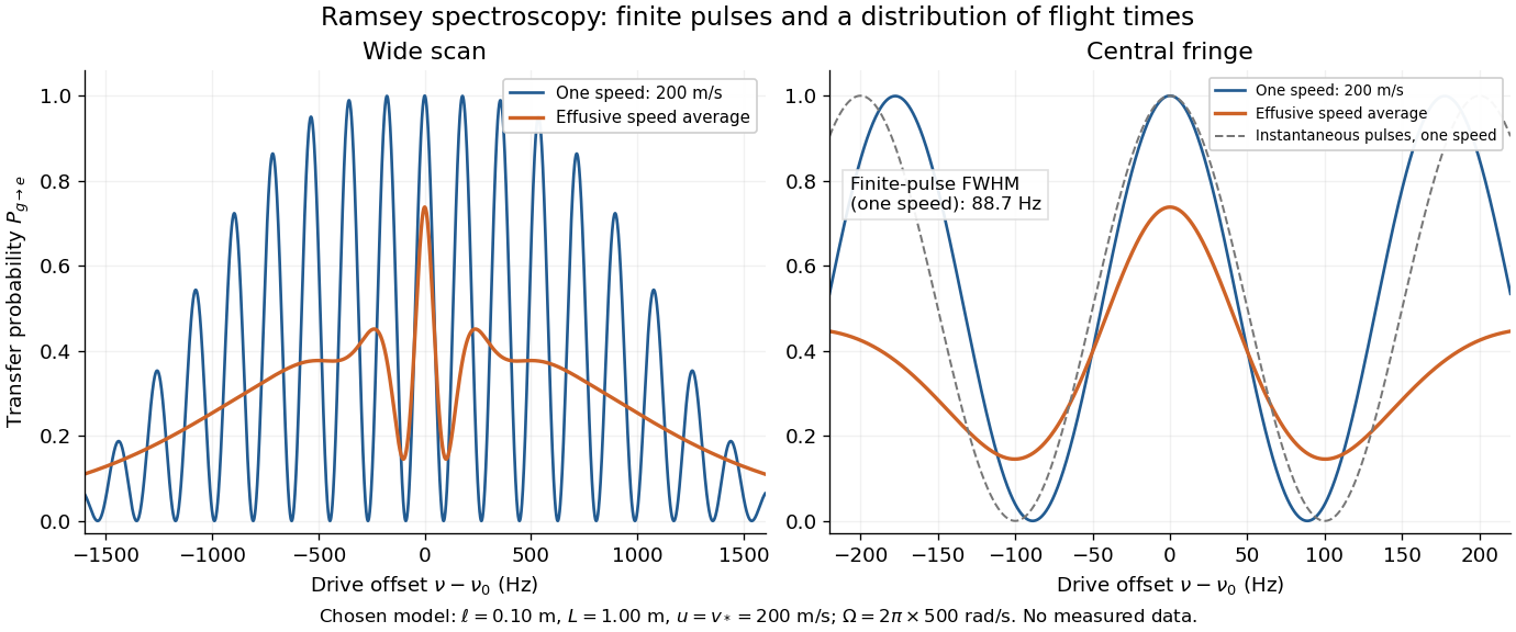
Different velocities smear side fringes because $\delta L/v$ varies across the beam. Nevertheless every term is even in $\delta$, so this symmetric ideal-model average has no odd line asymmetry that could displace the central lock point. Reduced contrast or altered width alone is not evidence of a shifted line center. A speed-dependent transition shift or unequal drive quantum phases changes that conclusion; atomic clock frequency shifts explains why these distinctions matter experimentally.

For an absolutely continuous distribution function with positive probability density function near its right endpoint of a distribution, write $\eta =f/(1-F)$ for its hazard function. The limits $t\eta (t)\to \alpha$ at an infinite endpoint or $(x_F-t)\eta (t)\to \alpha$ at a finite endpoint imply attraction to the Fréchet distribution or negative Weibull distribution, respectively. A continuously differentiable reciprocal hazard function with $(1/\eta {)}^{\prime }\to 0$ implies attraction to the Gumbel distribution, provided the survival function tends to zero at the endpoint.

The probability distribution of a nonnegative duration until an event. For a continuous duration with survival function $S(t)=P(T>t)$, its probability density function is $p(t)=-S^{\prime }(t)$. A constant hazard gives an exponential distribution; successive independent first-order waits give a convolution, as in the two-step catalytic waiting time.

For a probability density function $w$ on a domain, a weighted Poincare inequality has the formThe optimal $\lambda$ is the spectral gap of the associated weighted diffusion operator.

The unit-radius Wigner semicircle distribution has the displayed probability density function. Its graph is a rescaled upper semicircle. The area of the unit semicircle is $\pi /2$, so the factor $2/\pi$ normalizes it. Symmetry gives mean zero, and the substitution $x=\sin \theta$ gives variance $1/4$.

A scaled radius-$R$ version has density $2\sqrt{R^2-x^2}/(\pi R^2)$ on $(-R,R)$ and variance $R^2/4$. Rejection sampling from a uniform proposal on $(-1,1)$ accepts a proposed $x$ with probability $\sqrt{1-x^2}$; its average acceptance probability is $\pi /4$. Thus the number of proposals for one output has geometric distribution with expectation $4/\pi$. This law also describes the limiting empirical eigenvalue density in standard ensembles of large symmetric random matrices.