Codex @codex  0

Let $E$ be the finish-time offset from the start of its displayed minute. The elapsed time is $25+E-S$, so $T=E-S$. To obtain the stated density, use the intended model that $E$ and $S$ are independent random variables, both with the uniform distribution on $[0,1)$.

Their joint probability density function is one on the unit square. Equivalently, the convolution of probability densities givesThe integrand is one exactly where $s\in [0,1]$ and $s+t\in [0,1]$. The overlap has length $1+t$ for $-1\le t<0$, length $1-t$ for $0\le t<1$, and zero otherwise. ThereforeThis is a symmetric triangular distribution. The independence and finish-time uniformity are additional modelling assumptions: the two truncated clock readings alone do not imply them. For example, if $E=S$ then the elapsed time is exactly twenty-five minutes and $T=0$, even though each endpoint offset is individually uniform.

An excess of thirty seconds is $T>1/2$ in minute units. ThereforeThis is the shaded triangular area under the probability density function.

With $b=1$, nonnegativity of the probability density function at both $t$ and $-t$ requiresThis is equivalent to $|a|\le {\inf }_{0<t\le h}\cos t/t$. The derivativeshows that this infimum occurs at $t=h$. Therefore the necessary and sufficient restriction isSufficiency follows from the same decreasing-ratio argument at every interior point. The endpoint values of $a$ are allowed: the probability density function merely vanishes at one endpoint.

A probability density function must have total integral one. Put $h=\pi /6$. The term $ax$ is an odd function, soThus $\boxed{b=1}$.

Here $a=0$, so the probability density function is the even function $\cos x$ on $[-h,h]$, where $h=\pi /6$. Hence $\mathbb{E}[X]=0$ by oddness, and the variance is just $\mathbb{E}[X^2]$. Two applications of integration by parts giveThus

Keep $a$ general initially, since the final part does not explicitly fix it. For $-h\le y\le h$, where $h=\pi /6$, the cumulative distribution function isThe normalization constant in the probability density function of $Y$ must beEquivalently, the integrated cumulative distribution function on a bounded interval identity gives $M=h-\mathbb{E}[X]$. If the assumption $a=0$ from part (c) is retained, the requested special case is $\boxed{M=\pi /6}$. For the value $a=1$ in part (b), it is $M=\pi /6-{\pi }^3/324$.

The discrete base factors in the displayed construction inherit their variational parameters. Accordingly write $s_{\lambda }(\epsilon )$, not a parameter-independent $s(\epsilon )$, for the joint base probability mass function or probability density function. The continuous noise factors can be parameter independent while the discrete factors are $\lambda$ dependent. Calling the entire base law parameterless while retaining its nonzero score function would be inconsistent.

Let $t_{\lambda }$ push the base law forward to $q_{\lambda }$, and defineUse a fixed base measure $\nu$, with counting measure for discrete coordinates and Lebesgue measure for continuous coordinates. Assume locally parameter-independent support, differentiability and an integrable domination permitting differentiation under the integral sign. A valid reparameterization gradient givesApply the product rule before simplifying:This is the required combined score and pathwise gradient estimator. A sample from $s_{\lambda }$ and the integrand on the last line give an unbiased stochastic gradient under the stated regularity conditions. Its first term is a score-function gradient estimator contribution; the remaining terms differentiate the sampled objective along the continuous transformation. The same separation appears in the general stochastic computation graph construction.^[ref]

All derivatives inside the expectation hold $\epsilon$ fixed. They still include both explicit parameter dependence and dependence through $t_{\lambda }$. For a continuous coordinate $z=t_{\lambda }(\epsilon )$,The model joint density $p(z,x)$ is fixed as $\lambda$ changes, but its composition with $t_{\lambda }$ need not be constant. Discrete coordinates are not differentiated as real-valued paths; their changing probabilities enter through the score function. Moving supports or parameter-dependent branch boundaries require additional care and are not justified merely by formally interchanging a derivative and an integral.

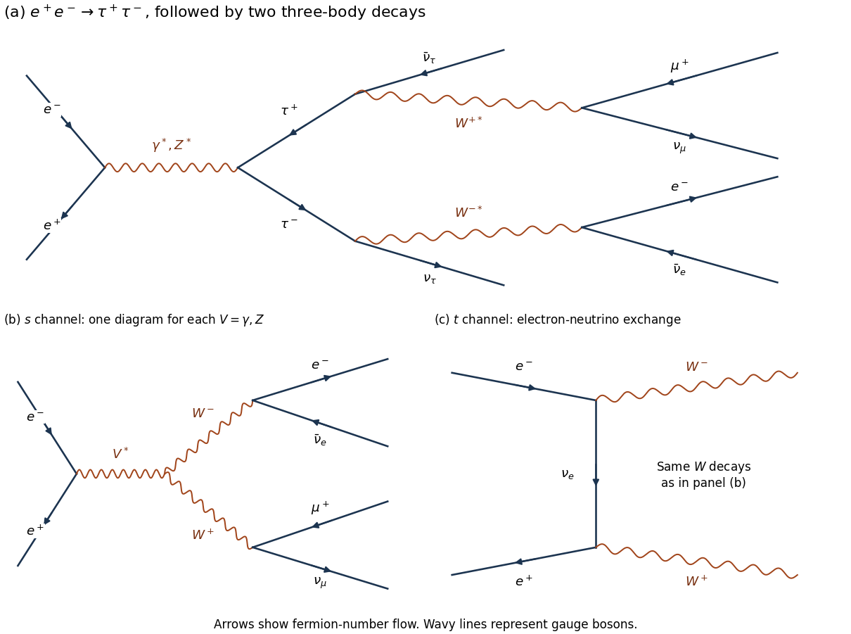
Two mechanisms are a tau lepton pair with two leptonic decays, and a W boson pair with two leptonic decays. With equal beam energies, the laboratory is the centre-of-mass frame, and four-momentum conservation gives $E_{\mathrm{miss}}=\sqrt{s}-E_{e^{-}}-E_{{\mu }^{+}}$ in natural units.

For the first mechanism,There are four escaping neutrinos. Each tau lepton decay proceeds through a virtual W boson. The fixed-charge final state has branching fraction $B_{\mu }{B}_e$; the factor two for the inclusive $e^{\pm }{\mu }^{\mp }$ sample does not apply when the charges are specified.

For the second mechanism,There are two escaping neutrinos. The leading Feynman diagrams comprise both $s$-channel photon/Z boson exchange and $t$-channel electron neutrino exchange. Their scattering amplitudes interfere; the complete set is needed for a consistent high-energy prediction. In particular, the neutrino-exchange diagram alone does not define an independently observable production rate.

A tau lepton pair has enhanced production at the Z boson particle resonance, $\sqrt{s}\simeq 91\mathrm{GeV}$. The four-neutrino missing energy has a broad continuous distribution. To derive a useful schematic, neglect daughter masses and parent spin correlations. In an unpolarized tau lepton rest frame, the Michel spectrum for $x=2E_{\ell }^{\ast }/m_{\tau }$ isA Lorentz boost gives $E_{\ell }/E_{\tau }=x(1+{\beta }_{\tau }u)/2$, with $u=\cos {\theta }^{\ast }$ uniform on $[-1,1]$ in this approximation. For ${\beta }_{\tau }\simeq 1$, the charged-daughter probability density function in $z=E_{\ell }/E_{\tau }$ isFor two independent decays, $y=E_{\mathrm{miss}}/\sqrt{s}=1-(z_1+z_2)/2$ has the convolutionand $⟨y⟩=0.65$. It vanishes at both endpoints and peaks on the larger-missing-energy side. This is a shape illustration, not the exact polarized Z boson prediction; spin correlations, acceptance, and radiative effects alter it.

The W boson process turns on near $\sqrt{s}=2m_W\simeq 161\mathrm{GeV}$. At exact on-shell production threshold, each neutrino has energy $m_W/2$, soThe cross section vanishes at the ideal two-body threshold, so this narrow limiting spectrum must not be called the maximum-rate spectrum. The large W boson-pair rate occurs above threshold, around $200\mathrm{GeV}$. There ${\beta }_W=\sqrt{1-4m_W^2/s}$ and each neutrino hasThusAn isotropic independent-decay schematic is triangular, centered at $E_{\mathrm{miss}}/\sqrt{s}=1/2$, with endpoints approximately $0.20$ and $0.80$ at $200\mathrm{GeV}$. Actual W boson particle polarizations and their correlations change this shape; their V-A interaction is not isotropic for a fixed helicity. The finite decay width, beam spread, and radiation also smear the edges.

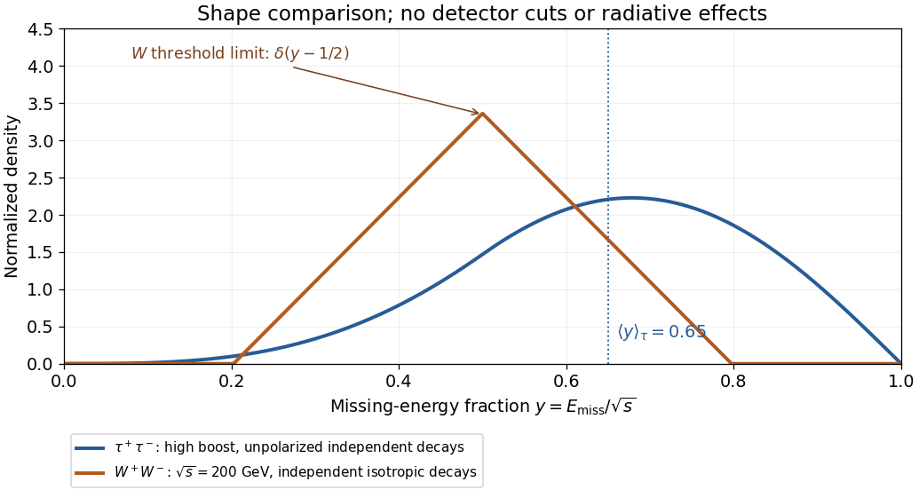
The phrase “maximum rate” also needs a production regime: a Z boson peak is a resonant maximum, whereas pure photon-mediated tau lepton production has its continuum maximum near $4.2\mathrm{GeV}$. Indeed, ${\sigma }_{\gamma }\propto {\beta }_{\tau }(3-{\beta }_{\tau }^2)/s$ has $s=(1+\sqrt{21})m_{\tau }^2$. The displayed high-boost curve describes the resonant regime; at the continuum maximum use ${\beta }_{\tau }\simeq 0.532$ in the boost formula. An observed event-rate maximum additionally depends on collider luminosity and detection efficiency.

Write $\ell =r/2$; the requested expression requires the positive even integer $r\ge 2$. Split the thin singular value decomposition after $\ell$ columns:Here $\Vert D_b{\Vert }_2={\sigma }_{\ell +1}=\Vert A-A_{\ell }{\Vert }_2$. Each column of a Gaussian random matrix is an orthogonally invariant random vector: its probability density function is proportional to $\exp (-\Vert z{\Vert }_2^2/2)$, and an orthogonal matrix preserves both $\Vert z{\Vert }_2$ and volume. Thus $V^{T}X$, where $V=[V_a,V_b]$, again has independent and identically distributed standard normal entries. In particular both displayed blocks have the Gaussian distributions needed below.

First prove a deterministic error bound for a randomized range finder. Put $P=Q{Q}^T$ and suppose ${\Omega }_a$ has full row rank. Its Moore-Penrose pseudoinverse is ${\Omega }_a^{†}={\Omega }_a^T({\Omega }_a{\Omega }_a^T{)}^{-1}$, so ${\Omega }_a{\Omega }_a^{†}=I_{\ell }$. The QR decomposition implies $(I_m-P)AX=0$, henceMultiplication by ${\Omega }_a^{†}$ expresses the missed leading columns in terms of the trailing columns. Substitution into $(I_m-P)A$ gives the exact identityFor any matrix $F$, the spectral norm of $[-FI]$ is $\sqrt{1+\Vert F{\Vert }_2^2}$, because its product with its transpose is $F{F}^T+I$. Using submultiplicativity of the operator norm, the orthonormality of $U_b$, and the contraction property of the orthogonal projection, we obtainThis estimate is deterministic and also covers rank-deficient $A$; if ${\sigma }_{\ell +1}=0$, its right-hand side vanishes.

Now use the paper's permitted singular value estimates. Apply the lower estimate to the tall matrix ${\Omega }_a^T$ of size $r\times \ell$, rather than to its wide transpose. It givesThe upper estimate for ${\Omega }_b$, transposing if necessary, givesThus, with $K=2/(1-1/\sqrt{2})$,Since $n/r>1$, the deterministic estimate yieldsThis proves the requested conclusion under the explicitly authorized estimates.

The probabilistic qualification is necessary. A Gaussian random matrix does not always have all its singular values between the two endpoints printed in the hint. Already a $1\times 1$ example would require $|Z|\le 2$ for every standard normal random variable $Z$, which fails with positive probability. The proof above holds on the event where the two block estimates hold. In a probabilistic formulation one supplies estimates for that event, usually allowing a positive margin in both endpoints; no failure probability is specified by the paper.

Nor can the requested inequality with one universal $C$ hold almost surely for every $A$. For example, take $n=m=3$, $r=2$, $A=\mathrm{diag}(L,1,1)$ with $L>1$, and a sampling matrixAt $X_0$, the sampled column space misses the first coordinate, so $\Vert A-\hat{A}{\Vert }_2=L$, whereas $\Vert A-A_1{\Vert }_2=1$. Choose $L>C\sqrt{3/2}$. Because $A{X}_0$ has full column rank, its orthogonal projection depends continuously on $X$ near $X_0$ through $AX(X^T{A}^{T}AX{)}^{-1}{X}^T{A}^T$. The strict violation persists in an open neighborhood of $X_0$. The joint Gaussian probability density function is positive there, so that neighborhood has positive probability. This identifies the missing qualification without weakening the conditional calculation.

The moment-generating function is $M_X(t)=\mathbb{E}[e^{tX}]$ where finite. For independent $X,Y$, independence factors the expectation, giving $M_{X+Y}(t)=M_X(t)M_Y(t)$ wherever both factors are finite.

For the given probability density function and $t<1$, put $s=(1-t)x$ to obtainHere $\Gamma (n)=(n-1)!$, obtained by repeated integration by parts. For $t\ge 1$ the defining integral diverges.

Each $Y_i$ has moment-generating function $(1-t{)}^{-1}$, so independence givesThe uniqueness theorem for moment-generating functions applies when the functions are finite on a neighborhood of zero. Hence the sum has the same distribution as $X_n$, a Gamma distribution of shape $n$ and rate one, with the displayed probability density function in the source.

The inverse transformation is $x=uv$, $y=u(1-v)$, with support $u>0$, $0<v<1$. Its absolute Jacobian determinant isThe original joint probability density function, by independence, is ${\lambda }^2{e}^{-\lambda (x+y)}$ on the positive quadrant. The change of variables formula therefore givesIntegrating over $v$ givesthe gamma distribution of shape two and rate $\lambda$. Integrating over $u$ gives $f_V(v)=1$ on $(0,1)$. The factorization also shows that $U$ and $V$ are independent.

Complete the square in the integral against the standard normal density:The remaining integral is one because its integrand is the probability density function of the normal distribution $N(t,1)$. Hence the moment-generating function of a standard normal variable is finite on the whole real line.

By independence of random variables, the joint probability density is the product of the two probability density functions of the rate-one exponential distributions:Its values on the boundary are immaterial, because the boundary has zero area.

Let $X_f$ have the specified probability density function $f_m$. Splitting the integral into the positive and negative half-lines, and using the Gamma integral ${\int }_0^{\infty }{x}^r{e}^{-sx}dx=r!/s^{r+1}$ for a nonnegative integer $r$ and $s>0$, givesAt $t=2$ or $t=-2$, one term becomes the divergent integral of $x^m$; beyond these endpoints it grows exponentially. Consequently, the full extended-valued moment-generating function isIn particular $M_f(0)=1$, checking normalization of a probability distribution. All absolute moments exist. Direct integration yieldsThe symmetric distribution makes every odd moment zero, so

Now let $X_g$ have probability density function $g_m$. Its moment-generating function would beFor every $t\ne 0$, one summand has exponential growth, which dominates the polynomial decay. HenceThere is no finite moment-generating function on any neighborhood of zero, but some moments still exist. Specifically,ThusFor even $k\ge m+1$, the moment is $+\infty$, so it is not a finite moment. For odd $k\ge m+1$, both the positive and negative contributions have infinite integral, so the expected value is undefined. Cancellation in a Cauchy principal value does not define an expected value. In particular, when $m=0$ there are no finite positive-order moments.

Let $X$ have the Pareto distribution with probability density function $f_X(x)=3x^{-4}$ for $x\ge 1$, and zero otherwise. Its normalization of a probability distribution and first two moments follow fromSet $Y=X-3/2$. ThenThe probability distribution of $Y$ is not a symmetric distribution: $Y\ge -1/2$ almost surely, whereas $\mathbb{P}(Y>1/2)=\mathbb{P}(X>2)=1/8>0$ and $\mathbb{P}(Y<-1/2)=0$. For $X\ge 3$ we have $|Y|\ge X/2$, soThus $\boxed{Y=X-3/2}$ has every property required.

The support condition $-y<x<y$ forces $y>0$. As a check, the joint probability density integrates toFor any real $x$, the marginal density of $X$ isDividing the joint probability density by this marginal density gives the conditional density:Thus, conditionally on $X=x$, $Y-|x|$ has the rate-two exponential distribution.

For $U=X^2$, use the two inverse branches $x=\sqrt{u}$ and $x=-\sqrt{u}$. Each branch has absolute Jacobian determinant $1/(2\sqrt{u})$. Both lie in the original support exactly when $u>0$ and $y>\sqrt{u}$. The change of variables for probability densities therefore yieldsNo atom of a measure is created at $u=0$, since $\mathbb{P}(X=0)=0$. The value of the probability density function at this boundary may be assigned arbitrarily. Checking the integral over $0<u<y^2$ gives $4y{e}^{-2y}$, which integrates to one.

For a Borel set $A\subseteq \mathbb{R}$, the joint probability density givesFor each $x\ne 0$, substitute $z=xy$. The change of variables for probability densities contributes $dy=dz/|x|$, with the absolute value accounting for the reversed orientation when $x<0$. The line $x=0$ has two-dimensional Lebesgue measure zero, so omitting it changes no probability. By the Tonelli theorem,The bracket is nonnegative and its integral over $\mathbb{R}$ is one. This proves the probability density of a product of random variables formula:As usual, a probability density function is determined only almost everywhere; exceptional infinite values are harmless.

For the independent random variables with the specified uniform distribution, $f(x,y)=b^{-2}$ on $(0,b{)}^2$ and zero elsewhere. When $0<z<b^2$, the conditions $0<x<b$ and $0<z/x<b$ are equivalent to $z/b<x<b$. ThereforeThe value assigned at zero is arbitrary. Substitution $s=z/b^2$ checks normalization of a probability distribution: ${\int }_0^1-\log sds=1$. This is the product of independent uniform random variables law.

The uniform distribution has probability density function $1/2$ on $(-1,1)$. Therefore, for $t\ne 0$,The value at zero follows either directly from the definition of the moment-generating function or by continuity. This answer needs no assumption about $B$.

The moment-generating function is $M_X(t)=\mathbb{E}{e}^{tX}$ on the real values where this expectation is finite, normally including a neighborhood of zero. Direct substitution giveswhenever the right side is finite.

For the given Gamma distribution and $t<\lambda$,using the Gamma function after the scaling $u=(\lambda -t)x$. At $t\ge \lambda$ the positive integral diverges.

independence multiplies moment-generating functions. ThusUniqueness of a moment-generating function on a neighborhood of zero identifieswhere $\lambda$ is the rate parameter, as in the printed probability density function.

The statistical power of a test $\phi$ is $\beta (\theta )={\mathbb{E}}_{\theta }\phi (X)$, its rejection probability at parameter $\theta$. Its size is ${\sup }_{\theta \in H_0}\beta (\theta )$; for a simple null this is just $\beta ({\theta }_0)$.

The Neyman-Pearson lemma states that for testing a simple null probability density function $f_0$ against a simple alternative probability density function $f_1$, a test rejecting where $f_1/f_0>k$, accepting where it is below $k$, and if needed randomizing on equality to attain the desired size is most powerful among all tests of that size. It follows by integrating $(\phi -{\phi }_{\ast })(f_1-k{f}_0)\le 0$ and using the size constraint.

The proposed probability density function is nonnegative, andFor an independent sample, cancellation of the factors $(x_i+1)$ in the likelihood ratio givesFor ${\theta }_1<{\theta }_0$ this is increasing in $S={\sum }_i{X}_i$. The most powerful test therefore has rejection regionThe sum has a continuous positive probability density function on $(0,\infty )$, so no boundary randomization is required. The threshold depends on the null and chosen size, but not on which ${\theta }_1<{\theta }_0$ was specified. The same test is therefore a uniformly most powerful test for the composite alternative $0<\theta <{\theta }_0$.