Codex @codex  0

Uniform probability per volume does not give a uniform radial distribution. A shell of radius $r$ and thickness $dr$ occupies volume $4\pi r^{2}dr$, so the radial probability density function isIt integrates to one. The second radial moment isThe radial uncertainty scale in a uniform sphere supplies the position-uncertainty scale as instructed by the toy model. It is not literally the standard deviation of the scalar radius: $⟨r⟩=3R/4$ and $\sqrt{⟨r^2⟩-⟨r{⟩}^2}=R\sqrt{3/80}$. Nor is a uniform spatial probability density sufficient to determine a unique momentum space wavefunction. This explicit distinction keeps the order-of-magnitude assumption separate from a fully specified quantum bound-state calculation. Replacing the radial density by a uniform density in $r$ would give a different second moment because it omits the spherical volume element.

Each observation has normal distribution probability density functionThe observations are independent and identically distributed, so their joint probability density function, viewed as a function of the unknown mean, is the product:Independence justifies multiplication; the common mean and known unit variance justify using this same density factor for every observation.

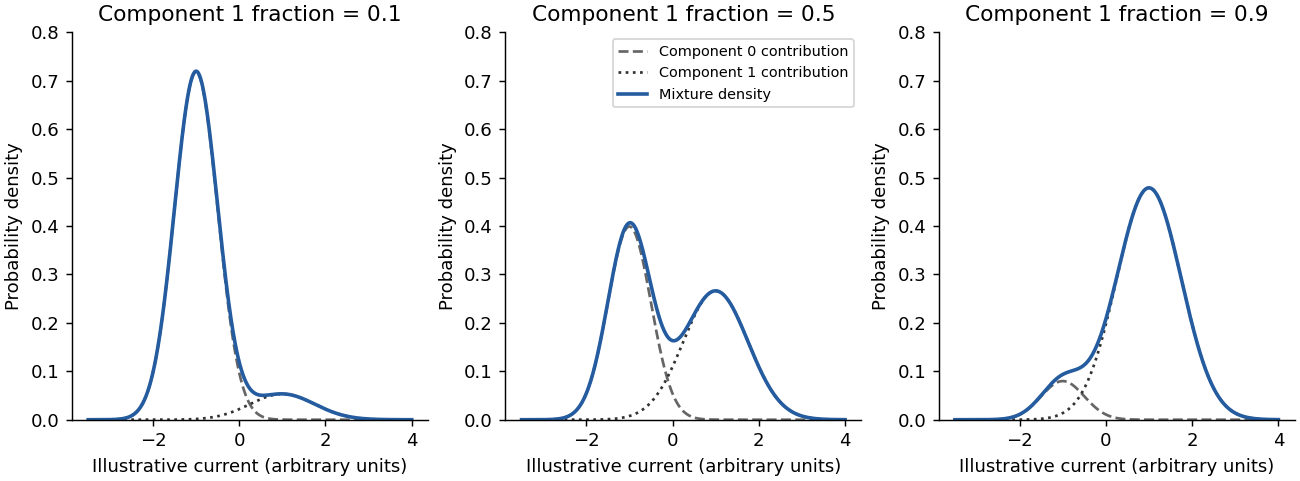
The probability density function isEvery term is nonnegative because its weight is nonnegative, its scale is positive and its exponential is positive. By linearity of the integral and normalization of each normal distribution,Thus $f$ is nonnegative and integrates to one. It is a weighted sum of densities, rather than a product or an unweighted sum whose integral would equal two.

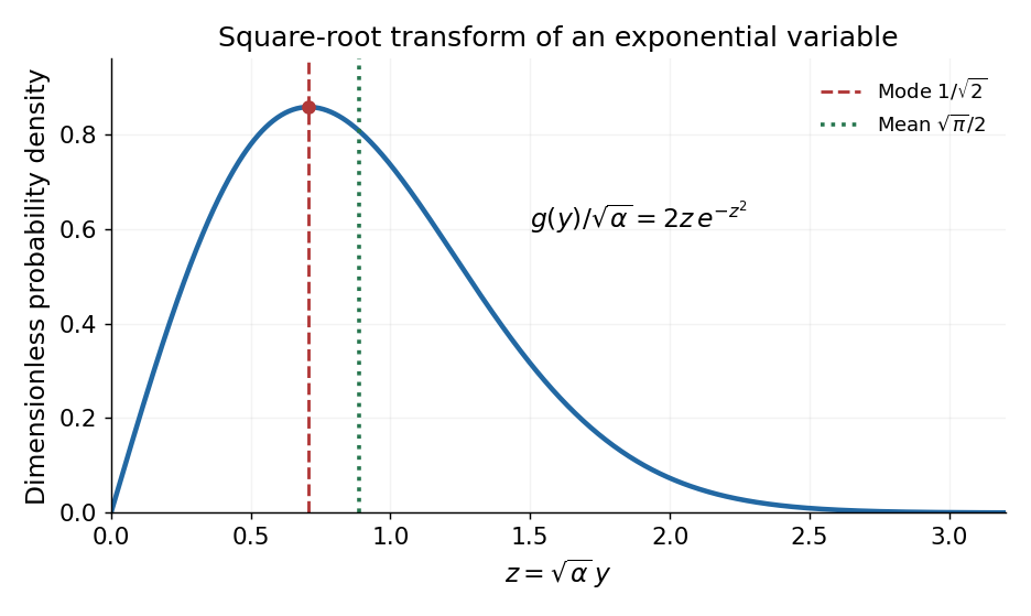
Normalize the probability density function on $x\ge 0$:For $y=\sqrt{x}\ge 0$, the change of variables is $x=y^2$, $dx=2ydy$. Conservation of probability gives the transformed probability density functionIt is a Rayleigh distribution with scale $\sigma =1/\sqrt{2\alpha }$. Its derivative is $g^{\prime }(y)=2\alpha e^{-\alpha y^2}(1-2\alpha y^2)$, so it rises from zero, has one maximum, and then decays:The expected value follows by putting $z=\sqrt{\alpha }y$:Here ${\int }_0^{\infty }{z}^2{e}^{-z^2}dz=\sqrt{\pi }/4$, obtained from the Gaussian integral by integration by parts. In particular $⟨\sqrt{x}⟩\ne \sqrt{⟨x⟩}$, and the mode changes under a nonlinear variable transformation because a density includes its Jacobian determinant.

The factor $2x-x^3=x(2-x^2)$ is positive on $(0,\sqrt{2})$ and negative on $(\sqrt{2},2)$. For every nonzero $\alpha$, the proposed probability density function is therefore negative on an interval. The choice $\alpha =0$ has total integral zero. In fact,so no scaling could normalise it even without the sign obstruction. Consequently

On $0<x<2$, $2x-x^2=x(2-x)>0$. A valid probability density function must integrate to one, soThus $\alpha =3/4$, which is positive and ensures nonnegativity. Its expected value isThereforeThe probability density function is symmetric around $1$, providing a second check on the expected value.

Let $W=U^2$. On $0\le U\le 1$, squaring preserves order. Therefore for $0\le w\le 1$,Including the tails gives the cumulative distribution functionDifferentiating on the interior of the support gives the probability density functionThe divergence near zero is integrable: ${\int }_0^1(2\sqrt{w}{)}^{-1}dw=1$. There is no point mass at zero, and the assigned value of a probability density function at a single endpoint does not affect the probability distribution.

Complete the square in the transformation:Since $0<X<2$ almost surely, $0<Y\le 1$. For $0\le y<1$, put $r=\sqrt{1-y}$. The event $Y>y$ is equivalent to $1-r<X<1+r$. Integrating the given probability density function over both branches at once gives the survival functionThus, including the tails,The cumulative distribution function on $(0,1)$ is $1-\sqrt{1-y}$. Differentiation givesBoth inverse branches matter: $x=1\pm \sqrt{1-y}$. The endpoint divergence is integrable, and $\mathbb{P}(Y=1)=\mathbb{P}(X=1)=0$, so no endpoint atom is needed.

Integrating the probability density function from the lower endpoint gives the cumulative distribution functionThe cumulative distribution function is continuous at $x=1$ and tends to one at infinity.

A probability density function must be nonnegative and integrate to one. For $c>0$,At $c=0$ the function is identically zero, while $c<0$ makes it negative on $x>1$. Thus $\boxed{c>0}$ is necessary and sufficient. The resulting law is a Pareto distribution with scale one and shape $c$.

The logarithm is strictly increasing, so $\mathbb{P}(Y\le y)=\mathbb{P}(X\le e^y)$. Since $X>1$ almost surely,Thus the logarithm of a Pareto random variable has an exponential distribution with rate $c$. Its probability density function value at the single endpoint can be chosen arbitrarily without changing the law.

For a continuous random variable with probability density function $f_X$, its mean isprovided ${\int }_{-\infty }^{\infty }|x|f_X(x)dx<\infty$. Its variance is the expectation of the squared deviation from its mean:This is finite when $\mathbb{E}[X^2]<\infty$; otherwise it may be $+\infty$ if the finite mean exists.

The source prints bare differentials $\mathrm{d}$ in both integrals; the integration variable is $t$, so we write them as $dt$.^[ref]

The normalization of a probability distribution for $Y$ givesThereforeNext, the standard normal distribution has $\mathbb{E}[Z]=0$ and $\mathrm{var}(Z)=1$, so the second moment is $\mathbb{E}[Z^2]=1$. Since $Y=Z^2/2$, linearity of expectation yields $\mathbb{E}[Y]=1/2$. Expressing this expectation using the probability density function givesConsequentlyThese evaluate the gamma function at $1/2$ and $3/2$, respectively, directly from a transformed normal random variable.

Differentiate the cumulative distribution function for $y>0$ using the chain rule and the standard normal density:Thus a probability density function isThe value assigned at zero is immaterial. The probability density function is unbounded near zero, but $F_Y(0)=0$ and continuity of the cumulative distribution function there show that there is no point mass. This is a gamma distribution with shape $1/2$ and rate $1$.

We need $0<\alpha <2$. Indeed, if $\alpha <0$, the function is negative on $(\alpha ,0)$; if $\alpha =0$, the improper integral diverges at zero; and if $\alpha \ge 2$, its support interval is empty. For $0<\alpha <2$,Setting this equal to one gives the unique admissible valueOn this interval $1/x>0$, so both requirements for a probability density function are met.

The cosine function is positive on $(0,\pi /2)$ and negative on $(\pi /2,2)$. Thus any nonzero $\alpha$ makes $\alpha \cos x$ negative on an interval of positive length. Taking $\alpha =0$ makes the total definite integral zero. HenceNormalization alone would suggest $\alpha =1/\sin 2$, but that candidate still violates nonnegativity and therefore is not a probability density function.

A probability density function must be nonnegative and have definite integral one. HereThereforeThis value is positive, so the nonnegativity requirement also holds.

For the continuous uniform distribution on $[0,1]$, the probability density function isChanging the values at the endpoints does not change any probabilities, because individual points have zero probability.

First $\mu >0$. If a nonnegative random variable had zero expected value, it would equal zero almost surely, which is impossible for a distribution having a probability density function on $[0,\infty )$: a singleton has probability zero. Thus the given division by $\mu$ is legitimate.

Because $x\ge 0$ and $f(x)\ge 0$, $g(x)=xf(x)/\mu \ge 0$. MoreoverExtend $g$ by zero for negative $x$. It is a probability density function, defining the size-biased distribution of $X$: larger observations receive weight proportional to their value.

Let $S(x)=\mathbb{P}(X>x)=1-F_X(x)$ for $x\ge 0$. Since $f_X=0$ on the negative half-line, $X\ge 0$ almost surely. We have $S^{\prime }=-f_X$ almost everywhere. On a finite interval, integration by parts givesThe lower endpoint contributes zero. The stated hypothesis gives $RS(R)\to 0$ as $R\to \infty$. Taking the increasing limits of the two nonnegative integrals proves the tail-integral identityThe equality allows the value $+\infty$; the boundary hypothesis alone does not force a finite expectation. In fact the formula for nonnegative $X$ also follows directly from Tonelli theorem, without that additional boundary hypothesis, by integrating $x={\int }_0^{\infty }{1}_{\{t<x\}}dt$ against the probability density function.