Codex @codex  0

For $x>\mu$, the corresponding smaller root is ${\mu }^2/x$. The conditional probability of selecting the larger root isIt is the same weight as a function of the actual selected value $x$. HenceCombining the two open intervals proves the output has the Inverse Gaussian distribution $IG(\mu ,\lambda )$. The event $Y=0$ has probability zero, so no atom occurs at $\mu$; the limiting density there is finite. The algorithm always selects one of its positive roots, so these branch densities exhaust its probability distribution.

Use the shape-rate convention for the gamma distribution. A shape $r$ and rate $\beta$ give expected value $r/\beta$ and variance $r/{\beta }^2$. The two moments here force $r=2$ and $\beta =2/\mu$. Thus $M_X(t)={\beta }^2/(\beta -t{)}^2$, and the geometric-sum moment-generating function becomesPut $r_0=\sqrt{1-p}$, $a=\beta (1-r_0)$ and $b=\beta (1+r_0)$. Then $0<a<b$, $ab=p{\beta }^2$, andConsequently the geometric sum of shape-two gamma variables has the same probability distribution as the sum of two independent exponential distributions with rates $a,b$. Their convolution of independent random variables yieldsThe probability density function is zero for $s<0$. It is nonnegative because $a<b$, and its integral isThis verifies normalization directly. An alternative check uses the conditional gamma distribution with shape $2n$:which is exactly the same density. The expected value $1/a+1/b=\mu /p$ supplies a further check.

Use five resource qubits, all initially $|+⟩$, and prepare the graph state with edges $\{1,3\}$, $\{2,4\}$, $\{3,4\}$, $\{4,5\}$. The labels here identify resource vertices; logical wire 1 travels from vertex 1 to 3, and logical wire 2 travels from 2 to 4 to 5. Each edge is a Controlled-Z gate, and these entangling gates commute, so all can be applied when preparing the resource.

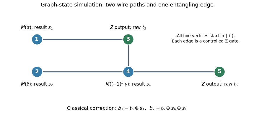
Measure vertex 1 in the equatorial qubit measurement basis at angle $\alpha$, with outcome $s_1$, and vertex 2 at angle $\beta$, with outcome $s_2$. These measurements can be simultaneous. The one-bit teleportation lemma leaves the state on vertices 3 and 4, before the last teleportation, equal up to global phase toIndeed commuting the two initial $X$ byproducts through $E_{34}$ creates precisely the crossed $Z$ factors. The unused edge from 4 to the fresh vertex 5 is the last one-bit teleportation link.

Measure vertex 4 at angle $\theta =(-1{)}^{s_2}\gamma$, with outcome $s_4$. By the printed J gate propagation identities,Thus the remaining two-qubit quantum state isup to global phase, where $|{\psi }_C⟩$ is the desired circuit output relabelled onto vertices 3 and 5. The sign choice cancels the unwanted angle reversal caused by the $X$ frame on vertex 4.

Finally measure vertices 3 and 5 in the computational basis, obtaining raw results $t_3,t_5$. The Pauli Z gate affects only phases, while the Pauli X gate flips a computational result. The five-vertex graph-state circuit simulation therefore outputsThis deterministic classical correction reproduces the ideal joint probability distribution for every preceding measurement branch. The final fixed-basis measurements may share the second layer with the adaptive measurement of vertex 4, because their projectors act on different vertices; measuring them afterwards is also valid.

The Quasi-Poisson regression retains the same conditional mean but permitsThis is a mean–variance function specification through quasi-likelihood; it does not assign a full probability distribution to each count. For independent observations, the quasi-score equation is proportional to ${\sum }_i{x}_i(Y_i-{\mu }_i)=0$, so the mean statistical parameter estimates equal those from Poisson regression. The output estimates $\hat{\varphi }=3.515351$ through the Pearson dispersion estimator, and inflates the standard errors by approximately $\sqrt{\hat{\varphi }}=1.875$.

The large residual deviance relative to 728 residual statistical degrees of freedom also signals substantial overdispersion. Daily weather, traffic and other omitted conditions may produce greater count variation than a homogeneous Poisson distribution allows. The Quasi-Poisson regression accounts for that extra marginal variance. It still requires a correct conditional mean and an appropriate independence assumption; a common dispersion parameter alone does not repair serial correlation.

A scoring rule in the reward convention gives $S(P,x)$ for announcing the probability distribution $P$ and then observing $x$. Under genuine belief $Q$, the expected score isA proper scoring rule satisfies $s(Q,Q)\ge s(P,Q)$ for every admissible $P,Q$. A strictly proper scoring rule additionally requires equality only when the distributions coincide:The expected scores must be well defined. A loss convention reverses the inequalities, but the question uses rewards.

Condition on the count and use the independence of random variables of the claim sizes. For $n\ge 1$ their joint exponential transform factors, while for $n=0$ the empty sum contributes $1$. Consequently the law of total expectation givesThis random sum of independent claims transform uses both independence assumptions: the count must be independent of the entire claim-size sequence, and the sizes must be mutually independent with the same probability distribution. The probability generating function is interpreted through its defining nonnegative series. The identity holds as a finite moment-generating function wherever that series is finite; outside that domain the expectation and series can agree at $+\infty$. In particular a positive argument may take $M_X(r)$ beyond $1$, so finiteness does not follow merely from the usual unit-disk domain of a probability generating function.

The moment-generating function of a mixture distribution is the mixture of its component transforms, soFor the aggregate, positivity of every claim implies $S=0$ exactly when $N=0$. ChooseIf $q>0$, take $\tilde{N}$ to have the zero-truncated claim-count distribution, namely the conditional law of $N$ given $N>0$. ThenChoose this count independently of a fresh independent claim-size sequence and put $Z={\sum }_{i=1}^{\tilde{N}}{X}_i$. Its probability distribution is that of $S$ conditional on being positive. Thus the hurdle decomposition of a positive random sum givesand an independent Bernoulli random variable $B$ of success probability $q$ realizes $S\stackrel{d}{=}BZ$. This establishes the distributional representation, including that $Z$ is itself a positive random sum of independent claims. If $p=1$, the aggregate is identically zero; set $q=0$ and choose any positive $Z$, for example one claim. Conditioning the count on positivity is then unnecessary and would be undefined.

For the specified geometric distribution on the nonnegative integers,An exponential distribution of expected value $\mu$ has transform $M_X(r)=(1-\mu r{)}^{-1}$. Substitution yieldsHence $Z$ is exponential with rate $1/(2\mu )$ and expected value $2\mu$. This is the geometric sum of exponential variables with a rescaling of the claim mean. Identification can also use the uniqueness theorem for Laplace transforms of nonnegative random variables by taking $r\le 0$.

The resulting distribution function isIts jump of size $1/2$ at zero is important: the aggregate law is not a purely continuous exponential distribution.

In an ontological model of a quantum system, a preparation of $|\psi ⟩$ gives a probability distribution ${\mu }_{\psi }$ over a physical state $\lambda$. A fixed quantum measurement has response probabilities ${\xi }_j(\lambda )\ge 0$ with ${\sum }_j{\xi }_j=1$, reproducing the Born rule after averaging over ${\mu }_{\psi }$. The PBR theorem says that, assuming preparation independence and the quantum predictions, distributions for distinct pure states cannot overlap with positive probability. Thus the quantum state is determined by the physical state in the psi-ontic model sense.

Preparation independence says that separately prepared systems have independent physical states: a product preparation is represented by the product of their individual ontic distributions. This is an assumption about the underlying physical states, not merely a statement that experimental preparation choices are independent. The excluded psi-epistemic model hypothesis is that the same physical state can occur with positive probability for two different pure-state preparations. The theorem neither excludes additional hidden variables nor claims that every interpretation which speaks of information is ruled out without these assumptions.

For the two given qubit preparations, consider the following PBR exclusion measurement for zero and plus, written in the ordered basis $00,01,10,11$:Direct inner products show that these four vectors are an orthonormal basis. Each labelled vector is orthogonal to the correspondingly labelled product preparation, so the associated projective measurement satisfiesThis is an example of antidistinguishable quantum states: every outcome excludes one possible preparation, although the preparations cannot be perfectly distinguished.

To prove the contradiction without requiring deterministic quantum measurement responses, choose a common dominating measure for ${\mu }_0,{\mu }_{+}$ and write their densities $m_0,m_{+}$. If they overlap, $\nu (\lambda )=\min (m_0,m_{+})$ has mass $\epsilon >0$. By preparation independence, every one of the four product densities dominates $\nu ({\lambda }_1)\nu ({\lambda }_2)$. Its total mass is ${\epsilon }^2$. The zero Born rule probability for outcome $xy$ implies that its nonnegative response ${\xi }_{xy}({\lambda }_1,{\lambda }_2)$ vanishes almost everywhere for its matching preparation, hence also under this common product measure. All four responses would then vanish on a set of positive measure, contradicting their sum being one. Therefore ${\mu }_0$ and ${\mu }_{+}$ are mutually singular.

For the second pair, group the $2n$ independent preparations into two blocks of $n$. Define $|{\Psi }_i⟩=|{\psi }_i{⟩}^{\otimes n}$. The tensor-power reduction of PBR overlap givesEach block therefore has an effective two-dimensional Hilbert space. Explicitly,are orthonormal and $|{\Psi }_2⟩=(|e_0⟩+|e_1⟩)/\sqrt{2}$. Embed the four-vector exclusion basis above into the tensor product of these two block spaces. To obtain a complete quantum measurement on all $2n$ qubits, add the orthogonal complement of that four-dimensional subspace to one of its four projectors. All four allowed preparations lie in the subspace, so the four forbidden probabilities remain zero.

If the single-copy preparation distributions overlap with common mass $\epsilon >0$, their $2n$-fold products all dominate the common measure ${\nu }^{\otimes 2n}$ of mass ${\epsilon }^{2n}>0$. The same zero-response contradiction now applies to the four block preparations. ThusThe argument is exact for the ideal devices specified in the question; no finite experimental resolution or noisy overlap bound is assumed.