Codex @codex  0

Daniel Tsui, Horst Störmer and Arthur Gossard reported the effect in 1982. They grew gallium arsenide–aluminium gallium arsenide layers by molecular beam epitaxy, separating the two-dimensional electron gas from its semiconductor doping. They cut Hall bars and made indium contacts. Low-field measurements established number density and charge carrier mobility. A perpendicular magnetic field sweep measured transverse and longitudinal sheet resistivities at several temperatures. Cooling sharpened the plateau near $3h/e^2$ and the longitudinal minimum at filling factor $1/3$; integer plateaus provided an internal comparison. The longitudinal minimum remained finite at the lowest temperature: zero-temperature vanishing was unresolved. This established anomalous transport, without directly measuring excitation electric charge.^[ref]

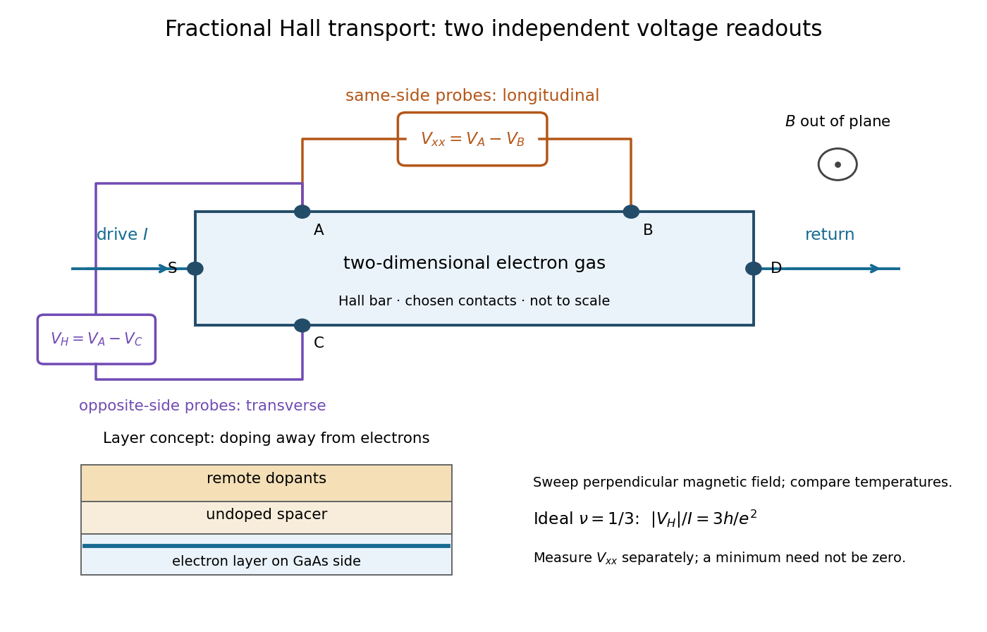
The two readouts test different statements. A single intersection with $R_H=3R_K$ would also occur on the smooth classical relation $R_H=B/(n_{s}e)$ at $n_{s}h/(eB)=1/3$. A quantum Hall plateau instead persists over a magnetic field interval. Comparing transverse and longitudinal signals helps distinguish that plateau from a contact-placement artefact; the quantum Hall conductivity tensor inversion quantifies the contamination when longitudinal sheet resistivity is nonzero.

Later, 1997 shot noise measurements associated with quantum tunnelling at filling factor $1/3$ tested the excitation electric charge separately, finding $e/3$. That is a different observable from a Hall plateau.^[ref]

Consider the original two-Electron example obtained by taking $N=2$ in the Laughlin wavefunction, with no additional polynomial for the centre of mass. Introduce $Z=(z_1+z_2)/2$, relative complex coordinate $w=z_1-z_2$, separation $r=|w|$, and dimensionless separation $u=r/{\ell }_B$. Since $|z_1{|}^2+|z_2{|}^2=2|Z{|}^2+|w{|}^2/2$, the probability density factorizes:Integrating out $Z$ leaves an isotropic relative probability density. Define $D_m(u)$ per unit dimensionless area and $p_m(u)$ per unit dimensionless separation:The physical areal probability density is $D_m(r/{\ell }_B)/{\ell }_B^2$. The probability of a separation between $r$ and $r+dr$ is $p_m(r/{\ell }_B)dr/{\ell }_B$. The extra $u$ comes from the Jacobian determinant in polar coordinates: a thin annulus has area $2\pi rdr$. Omitting that factor changes the question being answered.

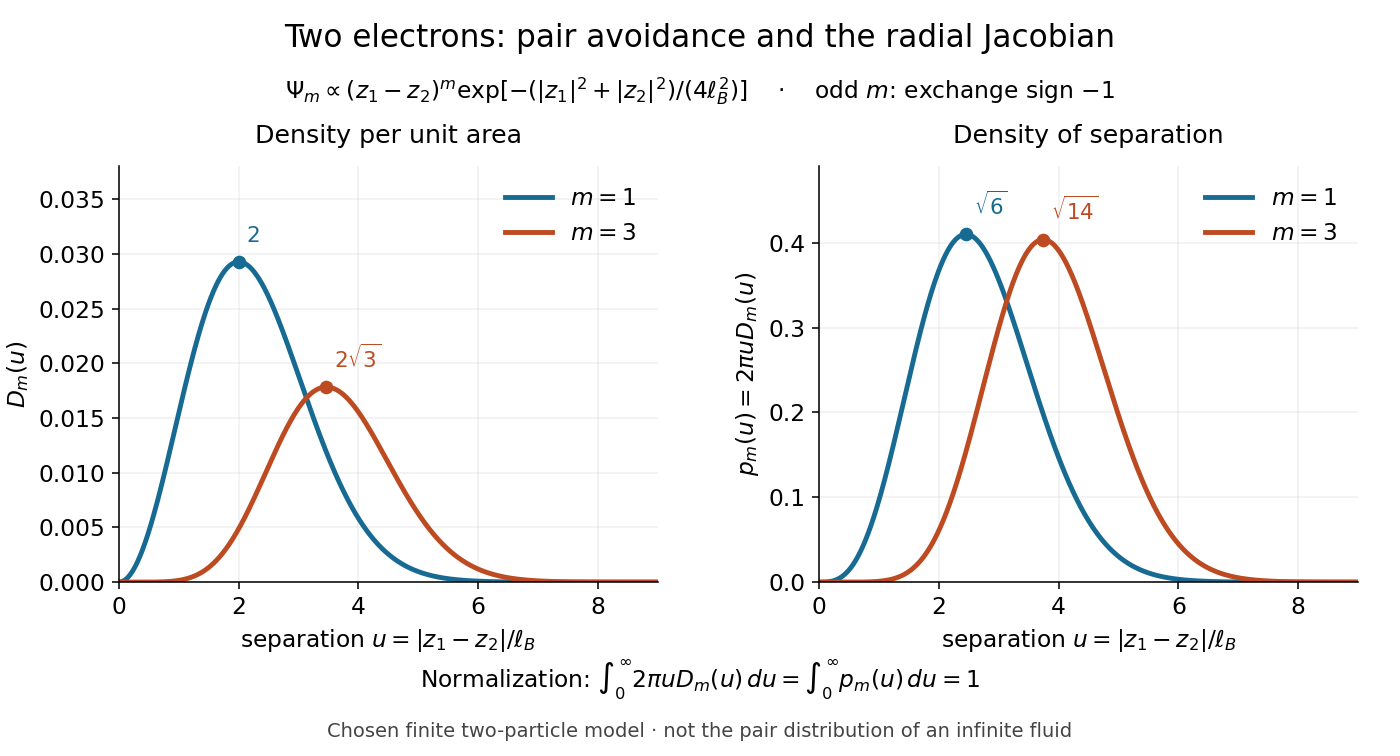
Both wavefunction normalization and the peak shift can be checked exactly. The substitution $t=u^2/4$ gives the Gamma function integralFor $m>0$, logarithmic differentiation givesConsequently the areal maximum lies at $u=2\sqrt{m}$, while the most probable separation lies farther out, at $u=\sqrt{4m+2}$. For $m=1$ these are $2$ and $\sqrt{6}\simeq 2.449$; for $m=3$, $\sqrt{12}\simeq 3.464$ and $\sqrt{14}\simeq 3.742$. The same substitution gives $⟨u^2⟩=4(m+1)$, so the root mean square separations are $\sqrt{8}$ and $4$ respectively. The distinction between a probability density maximum and a radial maximum therefore has a directly calculable geometric origin.

This two-Electron model explains exchange and pair avoidance. It does not establish a nonzero many-particle spectral gap, an extended quantum Hall plateau, or the topological properties of a fluid in the thermodynamic limit. Those require additional many-Electron reasoning and experimental tests.