Quantum Hall effect

The quantum Hall effect connects an electrical measurement to a quantum counting rule: a two-dimensional electron gas in a perpendicular magnetic field can exhibit plateaus of transverse electrical resistance. The integer case supplies a resistance scale built from the Planck constant and elementary charge, rather than the sample's dimensions. The fractional quantum Hall effect involves additional many-Electron physics.

On an ideal integer plateau, the magnitude of transverse sheet conductivity is $N{e}^2/h$, where $N$ is a positive integer, while the longitudinal sheet conductivity vanishes. The measured transverse electrical resistance is then $h/(N{e}^2)$. Both statements matter: inverting a conductivity tensor mixes its longitudinal and transverse components, as the quantum Hall conductivity tensor inversion shows.

The von Klitzing constant is $R_K=h/e^2=25812.807459\dots \Omega$. The current SI fixes the Planck constant $h=6.62607015\times 10^{-34}\mathrm{J}\mathrm{s}$ and elementary charge $e=1.602176634\times 10^{-19}\mathrm{C}$ exactly, so $R_K$ is exact; the displayed decimal is truncated. It differs from the historical conventional value $R_{K\text{-}90}=25812.807\Omega$.^[ref]

As an original ideal example, $N=2$ and electric current $I=1\mu \mathrm{A}$ give $|V_H|=I{R}_K/2\simeq 12.9064\mathrm{mV}$. Changing the Hall bar's width changes the transverse electric field required for this electric potential difference, while the ideal ratio $|V_H|/I$ remains $R_K/2$.

Klaus von Klitzing, G. Dorda and M. Pepper reported a silicon MOSFET measurement in 1980. Its gate controlled an semiconductor inversion layer; transverse contacts measured the Hall voltage and separate longitudinal contacts measured dissipation. One sweep held $B=18\mathrm{T}$, $T=1.5\mathrm{K}$ and $I=1\mu \mathrm{A}$ fixed while varying gate voltage. Hall plateaus accompanied small longitudinal voltages. Device-geometry comparisons and high-input-impedance voltage measurements helped test whether contact placement or electrical loading produced the result.^[ref]

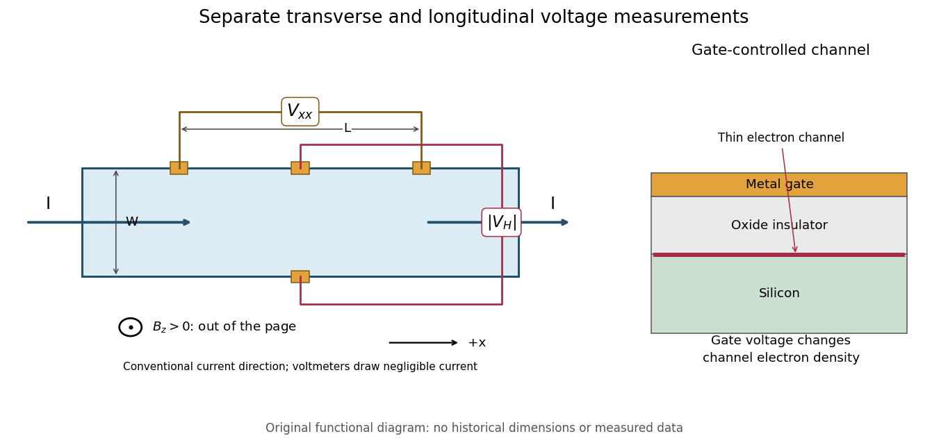
This original functional diagram separates transverse and longitudinal readouts; it does not reproduce the historical device's dimensions. The gate inset explains how a field-effect transistor provides an adjustable two-dimensional electron gas. A longitudinal voltage close to zero is a useful check because accidental longitudinal separation between Hall contacts can otherwise contaminate the transverse measurement.

A Hall bar is a strip with current contacts at its ends and additional voltage contacts along its sides. Opposite-side contacts measure a transverse electric potential difference; same-side contacts at different longitudinal positions measure a longitudinal electric potential difference. Separate voltage leads reduce the influence of current-contact electrical resistance when their input electric currents are negligible.

Voltage contacts separated along the current direction measure longitudinal resistance, even when the device is called a Hall bar. For an approximately uniform rectangular strip, $R_{xx}\simeq {\rho }_{xx}L/W$. Transverse contacts measure $R_{xy}$ instead. Shubnikov-de Haas effect oscillations in $R_{xx}$ need not be Hall-resistance plateaus; in the integer quantum Hall effect, longitudinal minima accompany quantized transverse plateaus.

The degeneracy of a Landau level is $eBA/h$ per resolved internal branch in area $A$. The filling factor $f=n_{s}h/(eB)$ varies continuously. Additional localized eigenstates need not carry bulk transport, allowing an integer plateau over an interval of $f$; a mobility gap need not be an empty spectral gap.^[ref]

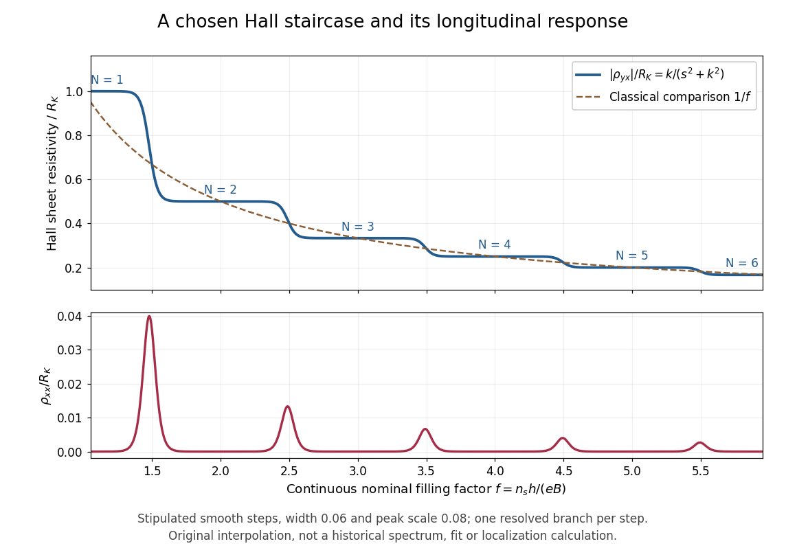
The plot is an original phenomenological construction, not measured data or a calculation of Anderson localization. It stipulates dimensionless transverse sheet conductivity $k(f)=1+\frac{1}{2}{\sum }_{m=1}^5[1+\tanh ((f-m-1/2)/w)]$ and longitudinal sheet conductivity $s(f)=a{\sum }_{m=1}^5{\mathrm{sech}}^2((f-m-1/2)/w)$, with chosen $w=0.06$, $a=0.08$. Both are measured in units $e^2/h$. The quantum Hall conductivity tensor inversion produces $|{\rho }_{yx}|/R_K=k/(s^2+k^2)$ and ${\rho }_{xx}/R_K=s/(s^2+k^2)$. Regions near $k=N$, $s=0$ yield plateaus near $R_K/N$; the model alone does not explain their microscopic robustness. Each step represents one resolved branch, without assuming unresolved spin or valley multiplicities.

Choose conventional surface current density along $+x$, magnetic field along $+z$, and negative Electron charge. An isotropic in-plane response has the following sheet conductivity and sheet resistivity tensors for $s\ge 0$, $k>0$:These are matrix inverses, rather than componentwise reciprocals. The sheet conductivity has units siemens, the sheet resistivity ohms. With $K_y=0$, the sign is $E_y/K_x<0$, agreeing with the negative Hall coefficient of a single Electron species. Contact polarity can reverse the measured voltage sign, so quote the Hall magnitude. For a homogeneous strip of width $W$ and longitudinal probe separation $L$, $I=W{K}_x$ givesAt $s=0$, $k=N$, these reduce to $R_K/N$ and zero. A nonzero transverse sheet resistivity creates no local Joule heating: the antisymmetric contribution cancels in $\mathbf{E}\cdot \mathbf{K}=(e^2/h)s|\mathbf{E}{|}^2$.

For an original nonideal example, choose $k=2$, $s=0.01$ and $L/W=2$. Then $V_{xx}/I\simeq 129.061\Omega$, while the Hall magnitude is below $R_K/2$ by the relative amount $s^2/(k^2+s^2)\simeq 25.0$ parts per million. An unwanted admixture $0.02V_{xx}$ in the Hall readout would instead introduce approximately $2.58\Omega$. The chosen calculation shows why a small intrinsic tensor correction does not by itself guarantee an accurate contact measurement.

For filled, separated, noninteracting magnetic Bloch bands, the Berry curvature integral over the magnetic Brillouin zone is an integer Chern number $C$, giving $|{\sigma }_{xy}|=|C|e^2/h$. Patches of Berry connection meet through phases with integer windings; continuous gap-preserving changes cannot change $C$. D. J. Thouless, M. Kohmoto, M. P. Nightingale and M. den Nijs developed this band argument; it does not establish the interacting fractional case.^[ref]

A quantum Hall edge state is confined across a boundary but can extend along it and carry electric current. B. I. Halperin related these current-carrying boundary states to quantized Hall transport in a disordered two-dimensional system.^[ref]

The fractional quantum Hall effect is quantized transverse sheet conductivity at fractional filling factors, produced by interacting Electrons. The Laughlin wavefunction describes the sequence $\nu =1/m$, with odd $m$, including $\nu =1/3$.^[ref]

For an original ideal readout example, take a Hall bar on the $\nu =1/3$ plateau with negligible longitudinal sheet conductivity. The quantum Hall conductivity tensor inversion givesHere $R_K$ is the von Klitzing constant; $R_H$ denotes transverse electrical resistance, rather than the bulk Hall coefficient. Thus a fractional sheet conductivity corresponds to a larger transverse electrical resistance. The fraction labels a collective quantum state: it does not mean that each Electron has acquired one third of its usual electric charge.

Daniel Tsui, Horst Störmer and Arthur Gossard reported the effect in 1982. They grew gallium arsenide–aluminium gallium arsenide layers by molecular beam epitaxy, separating the two-dimensional electron gas from its semiconductor doping. They cut Hall bars and made indium contacts. Low-field measurements established number density and charge carrier mobility. A perpendicular magnetic field sweep measured transverse and longitudinal sheet resistivities at several temperatures. Cooling sharpened the plateau near $3h/e^2$ and the longitudinal minimum at filling factor $1/3$; integer plateaus provided an internal comparison. The longitudinal minimum remained finite at the lowest temperature: zero-temperature vanishing was unresolved. This established anomalous transport, without directly measuring excitation electric charge.^[ref]

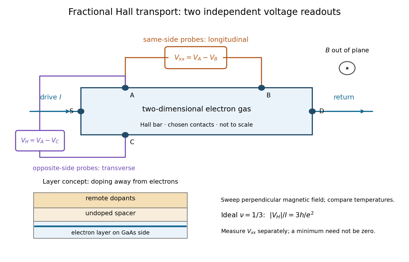
The two readouts test different statements. A single intersection with $R_H=3R_K$ would also occur on the smooth classical relation $R_H=B/(n_{s}e)$ at $n_{s}h/(eB)=1/3$. A quantum Hall plateau instead persists over a magnetic field interval. Comparing transverse and longitudinal signals helps distinguish that plateau from a contact-placement artefact; the quantum Hall conductivity tensor inversion quantifies the contamination when longitudinal sheet resistivity is nonzero.

Later, 1997 shot noise measurements associated with quantum tunnelling at filling factor $1/3$ tested the excitation electric charge separately, finding $e/3$. That is a different observable from a Hall plateau.^[ref]

Robert Laughlin's 1983 variational method uses pairwise zeros to suppress close Electron encounters within the lowest Landau level. For aligned spin, odd $m$ gives fermionic exchange symmetry.^[ref]

Here $\mathcal{N}$ enforces wavefunction normalization, ${\ell }_B$ is the magnetic length, and complex coordinates $z_j=x_j-i{y}_j$ describe Electrons in a magnetic field $B\hat{\mathbf{z}}$, $B>0$, with the symmetric gauge. Reversing the orientation conjugates the polynomial without changing probability densities. The Gaussian function confines the wavefunction.

The exchange check is especially simple for two Electrons. Writing $w=z_1-z_2$, exchange sends $w\mapsto -w$, so $w^m\mapsto (-1{)}^m{w}^m$. An aligned two-Electron spin state is symmetric, requiring the spatial wavefunction to change sign. Hence $m=1,3,5,\dots$ works, whereas $m=2$ would give the wrong sign. At a close encounter, the probability density vanishes as $|w{|}^{2m}$: $m=3$ imposes a sixth-order zero, stronger than the quadratic zero at $m=1$. This is the local geometric mechanism for avoiding a large repulsive Coulomb potential energy.

A useful large-$N$ counting outline follows directly from the polynomial. Each complex coordinate has maximum degree $m(N-1)$. A lowest Landau level orbital proportional to $z^k{e}^{-|z{|}^2/(4{\ell }_B^2)}$ has its areal probability density maximum at $r^2=2k{\ell }_B^2$, by differentiating its logarithm. This suggests droplet area $A\simeq 2\pi mN{\ell }_B^2$, neglecting the boundary correction. Dividing $N/A$ by the degeneracy of a Landau level per area, $1/(2\pi {\ell }_B^2)$, gives filling factor $\nu \simeq 1/m$. This counting is a motivation for the fraction, not an independent proof that the wavefunction minimizes the interacting Hamiltonian.

Consider the original two-Electron example obtained by taking $N=2$ in the Laughlin wavefunction, with no additional polynomial for the centre of mass. Introduce $Z=(z_1+z_2)/2$, relative complex coordinate $w=z_1-z_2$, separation $r=|w|$, and dimensionless separation $u=r/{\ell }_B$. Since $|z_1{|}^2+|z_2{|}^2=2|Z{|}^2+|w{|}^2/2$, the probability density factorizes:Integrating out $Z$ leaves an isotropic relative probability density. Define $D_m(u)$ per unit dimensionless area and $p_m(u)$ per unit dimensionless separation:The physical areal probability density is $D_m(r/{\ell }_B)/{\ell }_B^2$. The probability of a separation between $r$ and $r+dr$ is $p_m(r/{\ell }_B)dr/{\ell }_B$. The extra $u$ comes from the Jacobian determinant in polar coordinates: a thin annulus has area $2\pi rdr$. Omitting that factor changes the question being answered.

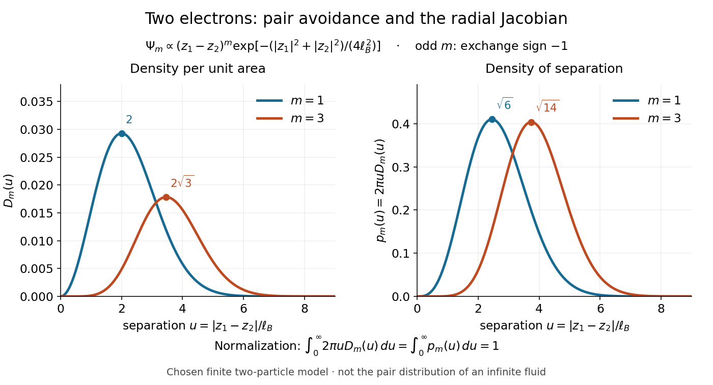
Both wavefunction normalization and the peak shift can be checked exactly. The substitution $t=u^2/4$ gives the Gamma function integralFor $m>0$, logarithmic differentiation givesConsequently the areal maximum lies at $u=2\sqrt{m}$, while the most probable separation lies farther out, at $u=\sqrt{4m+2}$. For $m=1$ these are $2$ and $\sqrt{6}\simeq 2.449$; for $m=3$, $\sqrt{12}\simeq 3.464$ and $\sqrt{14}\simeq 3.742$. The same substitution gives $⟨u^2⟩=4(m+1)$, so the root mean square separations are $\sqrt{8}$ and $4$ respectively. The distinction between a probability density maximum and a radial maximum therefore has a directly calculable geometric origin.

This two-Electron model explains exchange and pair avoidance. It does not establish a nonzero many-particle spectral gap, an extended quantum Hall plateau, or the topological properties of a fluid in the thermodynamic limit. Those require additional many-Electron reasoning and experimental tests.

A quasihole adds one zero at $\eta$ per Electron; its local deficit carries positive electric charge $e/m$.^[ref]

Here is a transport counting outline, conditional on an incompressible quantum Hall fluid. Inserting one magnetic flux quantum $\Delta \Phi =h/e$ slowly compared with $\hslash /\Delta$, where $\Delta$ is the excitation energy gap, produces a circulating electric field by Faraday's law. The transverse sheet conductivity sends a radial electric current whose time integral has magnitudeThe opposite electric charge moves to the boundary, so the total electric charge remains conserved. The counted deficit belongs to a collective quasiparticle; no individual Electron has been cut into pieces. The argument assumes the gapped fluid and its Hall response, and is not a consequence of the finite two-Electron normalization integral.

An incompressible quantum Hall fluid has a bulk spectral gap against charged excitations; disorder can localize excess quasiparticles.^[ref]