Codex @codex  0

Singularities. The complex exponential factors as $F(z)=e^{z/2}{e}^{1/(2z)}$. The second factor has an essential singularity at zero, and multiplication by the nonvanishing holomorphic function $e^{z/2}$ does not remove it. There are no other finite singularities. On the Riemann sphere, infinity is also an essential singularity, since $F(1/\zeta )=F(\zeta )$.

Symmetry and integral formula. The identity $F(1/z)=F(z)$ and uniqueness of the Laurent series on $0<|z|<\infty$ give $F_{-k}=F_k$ for every integer $k$. The Laurent coefficient formula, on the positively oriented unit circle, givesThe imaginary part vanishes by the substitution $\theta \mapsto 2\pi -\theta$. Hence

Polynomial contour integral. For an integer $n\ge 0$ and integer $p$, the binomial theorem gives $(1+z^2{)}^n={\sum }_{j=0}^n(\genfrac{}{}{0ex}{}{n}{j})z^{2j}$. The residue theorem selects $2j-n-p-1=-1$, that is $j=(n+p)/2$. Therefore the correct complete statement isThe printed nonnegative-integer condition alone misses $j\le n$. For example $n=0,p=2$ satisfies that condition, but the integral is zero and the displayed factorial $(-1)!$ is undefined.

Explicit coefficients. Both Taylor series inconverge absolutely and uniformly on every compact annulus away from zero, so their product can be regrouped. For $k\ge 0$, put $r=s+k$ and $s=m$. For arbitrary integer $k$, use the already proved symmetry:Here $I_j$ is a modified Bessel function. The printed series is directly meaningful for $k\ge 0$; for negative $k$ the absolute values, or an appropriately shifted lower summation limit, are essential.

Singularities and cuts. There are four simple poles $z_j=e^{i(\pi /4+j\pi /2)}$, $j=0,1,2,3$, because the roots of $1+z^4$ are simple and do not coincide with $\pm 1$. At $z=\pm 1$, the local behavior is a nonzero constant times $(z\mp 1{)}^{-1/2}$: these are square-root branch points. Infinity is not a branch point; on either branch $f(z)=O(z^{-5})$, so it extends there with a zero of order five. Three valid choices of branch cuts are the segment $[-1,1]$, the two rays $(-\infty ,-1]\cup [1,\infty )$ joined through infinity, or a semicircular arc joining $-1$ to $1$ and avoiding the poles. A circuit about either endpoint changes the sign, while a circuit about both endpoints does not.

Branch and residues. On $\mathbb{C}\setminus [-1,1]$, let $s(z)=\sqrt{z^2-1}$ be the branch with $s(z)/z\to 1$ at infinity, and define $\sqrt{1-z^2}=-is(z)$. Its upper boundary value on $(-1,1)$ is positive. The residue at a simple pole $z_j$ isFor fully explicit values, putIn counterclockwise order $z_0,z_1,z_2,z_3$, the values of $s$ are $A+iB,-A+iB,-A-iB,A-iB$. Since $A^2+B^2=\sqrt{2}$, substitution yieldsA branch point has no ordinary residue, since it has no single-valued Laurent series on a punctured neighborhood. At infinity the residue is zero.

Contour evaluation. The original contour goes counterclockwise around a large circle and clockwise round the slit, with its upper lip directed to the right. The large-circle contribution is $O(R^{-4})$. Small endpoint arcs contribute $O({ϵ}^{1/2})$. The artificial slit extension from $1$ to $R$ has equal boundary values on both sides, so its contributions cancel. On $(-1,1)$ the two boundary values of $f$ are opposite. Thus, with $I$ denoting the requested real integral, the residue theorem givesTherefore

For a positively oriented circle of any radius $R>0$, the residue theorem givesOnly the $z^{-1}$ coefficient in the Laurent series contributes. Reversing the orientation changes the sign.

If $f(z)=\sum a_j{z}^j$, then $f(-z)=\sum (-1{)}^j{a}_j{z}^j$ and its residue at zero is $-a_{-1}$. The circle $|z-1|=2$ encloses zero and no other finite singularity. Thus the residue theorem givesfor positive orientation.

Put $z=e^{i\theta }$, so $d\theta =dz/(iz)$, $\cos 2\theta =(z^2+z^{-2})/2$ and ${\cos }^{2}3\theta =(z^6+2+z^{-6})/4$. The contour integral isThe enclosed poles are $0$ and $\pm 1/\sqrt{2}$. For the rational function displayed without the prefactor $1/(4i)$, the residue at zero is $-21/8$ and the two other residues sum to $27/8$. Therefore the residue theorem givesA useful independent check is the Fourier series $(5-4\cos \varphi {)}^{-1}=\frac{1}{3}[1+2{\sum }_{k\ge 1}{2}^{-k}\cos k\varphi ]$; only its constant and third Fourier coefficients survive.

The coefficient of $z^{-1}$ in the Laurent series is $-1$. The residue theorem therefore gives, for the standard positive orientation,The residue theorem applies to an isolated essential singularity as well as to a pole.

Use the positive orientation shown in the source: the upper bank runs outwards and the lower bank returns towards one. On those banks the logarithm branch has values $\ell -i\pi$ and $\ell +i\pi$, respectively, with $\ell =\log (x-1)$. Their squared difference is $-4i\pi \ell$. The residue theorem therefore givesand henceThe large-circle contribution is $O(R^{-2}{\log }^{2}R)$ and the small circle about one contributes $O(\epsilon |\log \epsilon {|}^2)$, both tending to zero. These estimates justify replacing the closed contour integral by its two cut-bank integrals.

Let $I$ denote the requested integral. Symmetry and the period of ${\sin }^2\theta$ make the corresponding integral over $0\le \theta \le 2\pi$ equal to $4I$. With $z=e^{i\theta }$, this becomesThe denominator factors as $-2(z^2-1/2)(z^2-2)$. The two poles inside the unit circle are $z=\pm 1/\sqrt{2}$. Each residue is $1/(6i)$, because the derivative of the polynomial denominator there is $6z$. The residue theorem gives $4I=2\pi /3$, so

On the square, $|z|\ge N$. The identity $|\sin \pi (x+\alpha +iy){|}^2={\sin }^2\pi (x+\alpha )+{\sinh }^2\pi y$ bounds the sine away from zero on the vertical sides because $x=\pm N$; on horizontal sides it grows exponentially. Therefore the whole contour integral is $O(N^{-1})$ or smaller and vanishes. The residue theorem then giveswhich proves $\boxed{\sum _{n\in \mathbb{Z}}(-1{)}^n/(n-\alpha {)}^2={\pi }^2\csc \pi \alpha \cot \pi \alpha }$. Absolute convergence justifies the limiting residue sum.

Put $z=e^{i\theta }$, so $d\theta =dz/(iz)$, $\cos \theta =(z+z^{-1})/2$ and $\sin \theta =(z-z^{-1})/(2i)$. Rational expressions in these trigonometric functions become rational contour integrands on the unit circle. The method is especially useful when the resulting denominator has a small number of identifiable poles. A pole on the integration circle requires a separately specified principal value or indentation; the residue theorem does not automatically assign an ordinary integral there.

Put $z=e^{i\theta }$, so $\sin \theta =(z-z^{-1})/(2i)$ and $d\theta =dz/(iz)$. The integral becomesThe poles are $-2i/3$ and $-3i/2$; only the first is inside the unit circle. The derivative of the denominator there is $12(-2i/3)+13i=5i$. The residue theorem therefore givesThere are no poles on the contour because the real denominator is at least one.

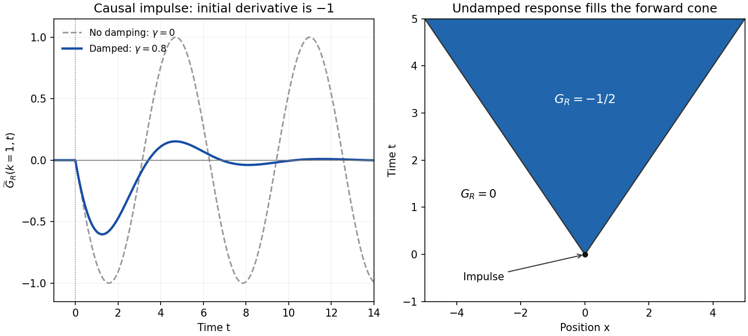
For $0<k^2<4/{\gamma }^2$, defineThe simple poles are ${\omega }_{\pm }=\pm {\Omega }_k-i{a}_k$. In the inverse transform $\tilde{G}(k,t)=\int e^{-i\omega t}\hat{G}d\omega /(2\pi )$, close the contour below for $t>0$. Its clockwise orientation gives $-i$ times the sum of residues. That sum isFor $t<0$, close above; there are no poles. The residue theorem therefore givesHere $\Theta$ is the Heaviside step function. At $k=0$ the continuous retarded limit is $-t\Theta (t)$. At critical damping, ${\Omega }_k\to 0$ likewise replaces $\sin ({\Omega }_{k}t)/{\Omega }_k$ by $t$; beyond the stated oscillatory range an imaginary ${\Omega }_k$ converts it to a hyperbolic sine. These continuations retain decaying temporal exponents.

For each fixed $k$, taking $\gamma \to 0^{+}$ givesFor $t>0$, invert in space and set $s=kt$:The correctly normalized sinc function transform isFor instance, $\sin s/s=\frac{1}{2}{\int }_{-1}^1{e}^{isy}dy$, and Fourier inversion immediately gives the factor $\pi$. The PDF's prefactor $\sqrt{2/\pi }$ is inconsistent with its top hat of unit height; it would give height $\sqrt{2\pi }$. Using the normalized identity yieldsas a distribution. The values assigned precisely at a wave front do not change that distribution. This is the negative of the standard one-dimensional retarded wave Green function, because the PDF's differential operator is $-{\partial }_t^2+{\partial }_x^2$.

The sign and initial data can be checked without any contour calculation. Integrating the spatial-Fourier equation through the impulse givesIn real space these are $G_R(x,0^{+})=0$ and ${\partial }_t{G}_R(x,0^{+})=-\delta (x)$. In particular,for a smooth test function $f$, confirming the negative delta-function initial velocity. Before the impulse the displacement and velocity are zero. The disturbance fills the forward causal cone for the constant-speed wave equation, whose fronts move at unit speed, consistent with $\rho =\kappa =1$. The final question's printed $\rho =k$ is interpreted as $\rho =\kappa$, referring to the elastic constant, not to the Fourier wavevector. No initial conditions were otherwise specified, so the causal choice has been made explicitly.

For real $a>b>0$, put $d=\sqrt{a^2-b^2}$. The change of variables $z=e^{i\theta }$ changes the integral to ${\oint }_{|z|=1}(2/b)dz/[z^2+2i(a/b)z-1]$. The roots are $-i(a-d)/b$ and $-i(a+d)/b$, with only the first inside the circle because $a-d=b^2/(a+d)$. The residue there is $1/(id)$, and the residue theorem proves the displayed result. A shift of the angular variable replaces sine by cosine. More generally for real $a>|b|$, the same answer follows by shifting by $\pi$ when $b<0$, and the case $b=0$ follows directly.

For $0<a<1$, integrate $e^{az}/(1+e^z)$ around a rectangle of imaginary height $2\pi$. Its single pole at $\pi i$ has residue $-e^{\pi ia}$, the top-edge integral is $-e^{2\pi ia}$ times the bottom-edge integral, and both vertical sides vanish at large real width. The residue theorem gives ${\int }_{\mathbb{R}}{e}^{ax}/(1+e^x)dx=\pi /\sin (\pi a)$. Substitution $t=e^x$ gives the equivalent integral ${\int }_0^{\infty }{t}^{a-1}/(1+t)dt$.

The residue of a function $f$ at an isolated singularity $a$ is its Laurent coefficient of degree $-1$. More explicitly, if $f$ is holomorphic for $0<|z-a|<\rho$, write its Laurent series asThis one Laurent coefficient determines the contour integral around a sufficiently small counterclockwise circle about $a$. A complicated local Laurent series can therefore leave a remarkably simple answer after one complete trip around the point.

For a simple pole, multiplying by $z-a$ removes the pole, leaving a holomorphic extension whose value at $a$ is the residue:There is a useful shortcut for a quotient $f=g/h$. If $g$ and $h$ are holomorphic near $a$, $h$ has a simple zero there, and $g(a)\ne 0$, then $f$ has a simple pole andThe first-order Taylor series of $h$ explains the denominator: dividing $h(z)$ by $z-a$ leaves its derivative at $a$ in the limit. This computes a residue without finding the full Laurent series, which is especially useful when the numerator or denominator is complicated. ^[ref]

For example, the rational function $f(z)=1/(z^2+1)$ has simple poles at $i$ and $-i$. Factoring the denominator makes both residues immediately visible:The signs matter: these residues cancel when both poles are enclosed, but either one contributes when enclosed alone. The residue theorem below turns this distinction into different contour integrals of the same function.

A residue is not the same thing as a pole, nor does it measure the order of a pole. The function $1/z^2$ has a double pole at zero but residue zero. Conversely,has an essential singularity at zero and residue one. Infinitely many negative powers cause no difficulty in reading off that particular Laurent coefficient. At a removable singularity the residue is zero. ^[ref]

Why does only this Laurent coefficient survive? Parametrize a counterclockwise circle by $z=a+r{e}^{it}$, $0\le t\le 2\pi$, with $0<r<\rho$. For every integer $n$,When $n\ne -1$, the complex exponential completes a whole number of turns and its contributions cancel; when $n=-1$, it is constant. Uniform convergence of the Laurent series on this circle justifies termwise integration, giving $\oint f(z)dz=2\pi i\mathrm{Res}(f,a)$. Thus the residue isolates exactly the local information that a closed contour integral detects. ^[ref]

This selection rule explains why a very large value near an isolated singularity need not produce a large contour integral. The double pole $1/z^2$ grows faster near zero than $1/z$, yet its contributions around a circle cancel completely. What matters is the arrangement of complex values along the path, including the differential $dz$, rather than their moduli alone. A residue records that surviving contribution, not the size of the function near the point.

Let $\Gamma$ be a piecewise smooth contour forming a simple closed curve, positively oriented: travel counterclockwise, with the interior on the left. Suppose $f$ is holomorphic on an open set containing $\Gamma$ and its interior, except at finitely many isolated singularities $a_1,\dots ,a_m$ strictly inside. ThenNo isolated singularity may lie on $\Gamma$: the ordinary contour integral must be defined there. Reversing the direction of the contour reverses the sign of the answer. The theorem applies to essential singularities as well as poles. ^[ref]

Return to $f(z)=1/(z^2+1)$. A counterclockwise circle $|z|=2$ encloses both simple poles, soYet $f$ is nonzero everywhere it is defined. A zero contour integral does not imply a zero function, or even absence of poles: the enclosed residues can cancel. By contrast, the counterclockwise circle $|z-i|=1/2$ encloses only $i$, givingThe picture compares these two selections. Changing the shape of a contour while keeping the same enclosed poles leaves the contour integral unchanged, provided the contour deformation stays where $f$ is holomorphic.

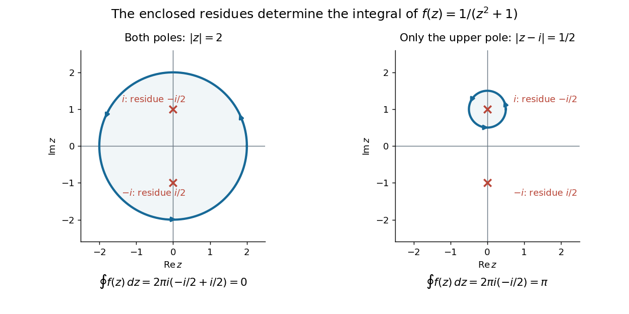
This is the practical appeal of the residue theorem: local Laurent coefficients determine a global contour integral. For a rational function, a few simple pole computations can replace a long parametrized calculation. It also makes real improper integrals accessible by treating the real line as part of a closed contour in the complex plane.

To compute $I={\int }_{-\infty }^{\infty }dx/(1+x^2)$, take $R>1$ and travel along the real line from $-R$ to $R$, then return along the upper semicircle $A_R$, parametrized by $z=R{e}^{it}$ for $0\le t\le \pi$. This contour is positively oriented and encloses the simple pole $i$ only; $-i$ is outside. HenceThe added arc must be controlled before taking a limit. On $A_R$, the reverse triangle inequality gives $|z^2+1|\ge R^2-1$, and the arc length is $\pi R$. The estimation lemma therefore yieldsThe denominator grows quadratically while the arc length grows only linearly. This quantitative comparison, rather than a sketch alone, explains why closing the contour does not alter the limiting real improper integral. It even supplies an error bound: the difference between $\pi$ and the finite real integral is at most $\pi R/(R^2-1)$.

For a numerical check, $R=10$ gives the finite real integral $2\arctan (10)\approx 2.94226$, leaving about $0.19934$ to reach $\pi$. The arc bound is $10\pi /99\approx 0.31733$, comfortably larger than that error. The graph shows both quantities approaching zero. The exact tail here can be checked with the antiderivative $\arctan x$; the residue theorem method remains useful for improper integrals where a convenient real antiderivative is unavailable.

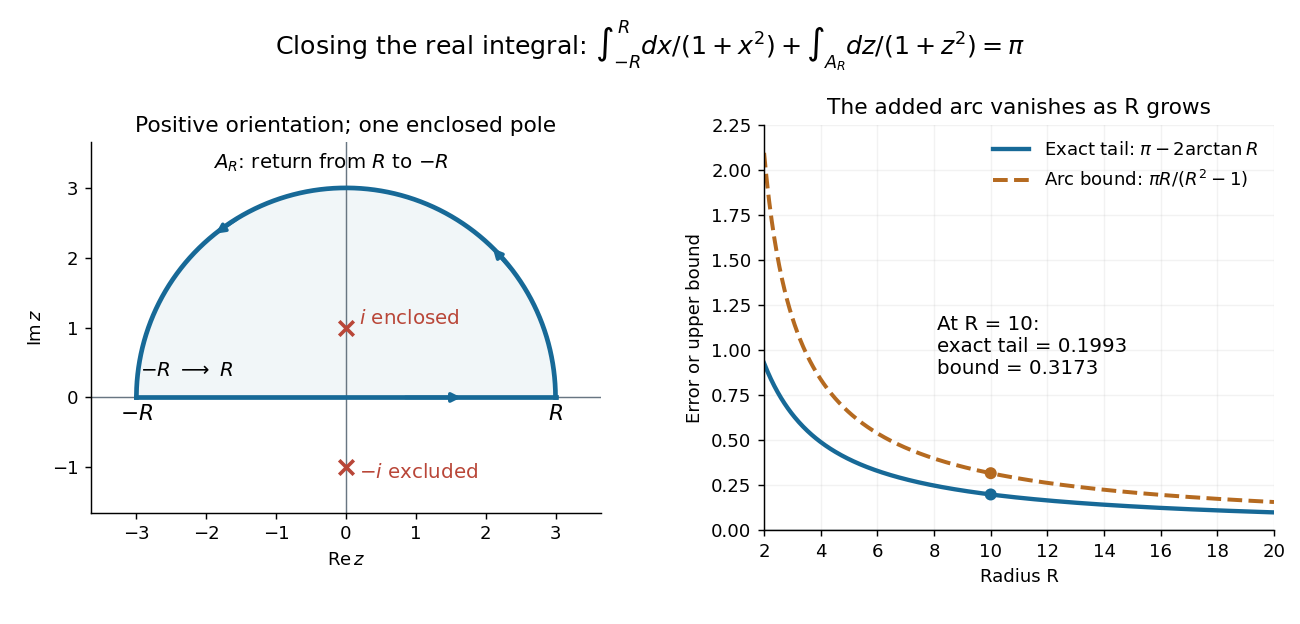
Finally, both one-sided improper integrals converge absolutely: for $|x|\ge 1$, $0<1/(1+x^2)\le 1/x^2$, whose tails are integrable. Thus the symmetric limit computes the ordinary improper integral, not merely a Cauchy principal value, andClosing below instead would enclose the simple pole $-i$. With the same left-to-right traversal of the real line, that contour is clockwise, so its contour integral is $-2\pi i\mathrm{Res}(f,-i)=\pi$ again. This provides a useful sign check: the opposite residue is accompanied by the opposite direction around the enclosed region.

The same strategy extends to many other rational functions: choose a contour, identify its enclosed isolated singularities, compute their residues, and bound the added pieces. The choice of contour and the bound are as much part of the calculation as the residues. ^[ref]

For $P(z)=a_N{z}^N+\cdots +a_0$ with $N\ge 1$ and $a_N\ne 0$, the unique retarded fundamental solution is $E=Hu$, where $P(D)u=0$, $u^{(j)}(0)=0$ for $j<N-1$, and $u^{(N-1)}(0)=1/a_N$. The distributional jump formula for a Heaviside product gives $P(D)E={\delta }_0$. Its explicit expression isThe residue theorem gives the initial derivatives from the coefficients at infinity. Equivalently, the inverse Fourier transform is integrated below all its poles, producing support of a distribution in $[0,\infty )$. Uniqueness follows because the difference of two retarded solutions is an analytic homogeneous solution vanishing on the negative half-line.

With ${\Delta }_F=⟨0|T\{\varphi (x)\varphi (y)\}|0⟩$, for a mode of positive energy $E>0$ the Feynman i-epsilon prescription puts poles $+E-i0$ and $-E+i0$ in opposite half-planes. The energy contour integral closes clockwise below for positive time separation and counterclockwise above for negative separation. The residue theorem gives $e^{-iE|t|}/(2E)$ in either case. Thus the four-dimensional Fourier integral has numerator $i$ and denominator $p^2-m^2+i0$. The integral is understood as a distribution limit, not an ordinary absolutely convergent integral; changing the definition to $i{\Delta }_F$ would change the displayed normalization.

Let $a>0$ and let $R$ be a rational function with $R(z^2)$ finite for real $z$ and $R(u)=O(u^{-1})$ at infinity. Choose the branch $h(z)=\sqrt{z^2-a^2}$ analytic off $[-a,a]$, with $h(z)\sim z$ at infinity. Put $g(z)=zR(z^2)/h(z)$. On the real exterior, $g(-x)=g(x)$; on the upper bank of the cut, $h(x+i0)=i\sqrt{a^2-x^2}$, so $g(x+i0)$ is odd in $x$.

Close a real-axis contour with a large upper semicircle, making clockwise upper indentations at the two branch points. The large arc vanishes because $g=O(z^{-2})$. Each small indentation is $O(\sqrt{\epsilon })$ and vanishes. The integral along the upper bank of $[-a,a]$ is zero by oddness; the two exterior pieces sum to twice the required integral. The residue theorem therefore givesResidues must use the chosen branch, notably $h(iy)=i\sqrt{y^2+a^2}$ for $y>0$. The substitution $u=\sqrt{x^2-a^2}$ provides an independent real-variable check, converting the integral to ${\int }_0^{\infty }R(u^2+a^2)du$.

By Jeremy Orloff, named on the first page of the notes for MIT 18.04, Complex Variables with Applications, Spring 2018. The credit here refers to this authored set of notes.

Official course resource: ocw.mit.edu/courses/18-04-complex-variables-with-applications-spring-2018/resources/mit18_04s18_topic11/

Online text: ocw.mit.edu/courses/18-04-complex-variables-with-applications-spring-2018/44f1db513a6a17d655abe0b6ff7748fc_MIT18_04S18_topic11.pdf

Cited passages: §11.2, Theorems 11.1 and 11.4, pp. 1–3, gives the argument principle and its residue theorem explanation; §11.2.3 covers Rouché's theorem; §11.3.6 explains the Nyquist stability criterion, including the sign from the clockwise contour used there. Our rational-function and sparse-sampling examples and images are independently calculated.