Codex @codex  0

Catherine A. Rychert and Peter M. Shearer used fifteen years of global seismic wave observations to image a sharp interface near the lithosphere-asthenosphere boundary. Conversions from P waves to S waves constrain the interface's depth and sharpness: a transition that preserves high-frequency converted phases is too sharp to be explained by a broad thermal gradient alone. Their interpretation therefore considers composition, melting and seismic anisotropy, and distinguishes the interface beneath oceans from a possible internal boundary inside thicker cratons.^[ref]

A seismology researcher studying lithosphere and asthenosphere structure. Institutional profile: mit.whoi.edu/faculty/5644/

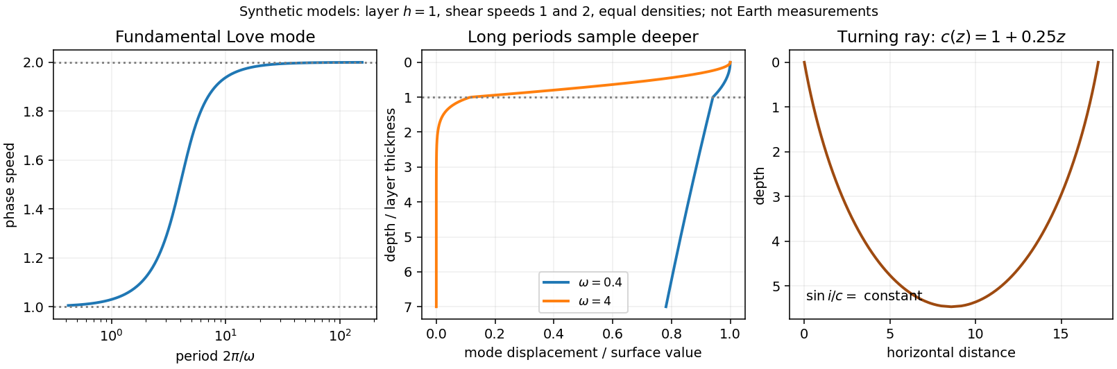
Seismic surface-wave dispersion. Rayleigh waves combine vertical and longitudinal motion in the vertical plane of propagation; Love waves have horizontal transverse motion and can be guided by a low-shear-speed surface layer. A homogeneous elastic half-space supports a Rayleigh wave with a frequency-independent speed in the ideal elastic limit, but depth-dependent Earth structure makes the surface-wave eigenfunctions and their propagation speeds depend on frequency. This structural dispersion can occur even when each constituent material is itself nondispersive.

Distinguish phase velocity $c=\omega /k$ from group velocity $U=d\omega /dk$, which controls a narrow-band envelope in the appropriate weakly attenuating limit. Longer periods generally have deeper sensitivity, while shorter periods emphasize shallower structure. In a profile whose shear speed increases with depth this often makes long-period waves faster, but low-velocity zones, anisotropy and higher modes can change that trend. Frequency dependence need not be monotonic in every Earth model.

Measure phase delays or wave-packet arrival times across known source–receiver paths for many periods, accounting for source phase, cycle ambiguity, multipathing and mode identification. Compute predicted dispersion from trial elastic profiles and compare with observations. Linearization expresses the sensitivity schematically aswhere $\alpha ,\beta$ are compressional and shear speeds. A regularized inverse problem then estimates depth structure; many crossing paths additionally provide surface-wave tomography. Joint Love wave and Rayleigh wave measurements help distinguish shear-wave polarizations and constrain radial seismic anisotropy. Finite bandwidth, depth averaging and correlated sensitivities mean that one dispersion curve does not uniquely determine a detailed Earth profile.

Seismic ray theory, the eikonal equation and Fermat's principle. In a smoothly varying isotropic medium, insert a high-frequency ansatz $u=A(\mathbf{x})e^{i\omega [T(\mathbf{x})-t]}$ into the scalar wave equation. The leading powers of frequency giveThe travel-time surfaces are wavefronts and rays are their normal trajectories, with slowness vector $\mathbf{p}=\nabla T$. The next-order equation transports amplitude, including geometrical spreading; attenuation is an additional material effect.

Fermat's principle says that the ray makes $\int ds/c$ stationary under path variations with fixed endpoints. Stationarity, rather than always the global minimum, permits multiple arrivals. Its Euler–Lagrange equation, with arclength $s$ and unit tangent $\hat{\mathbf{t}}$, isFor horizontal layering, the horizontal slowness $p_h=\sin i/c$ is conserved, giving Snell's law at interfaces and smooth refraction between them. Here $i$ is measured from vertical. A turning point satisfies $p_{h}c(z)=1$; increasing speed with depth bends a downgoing ray back upwards. Travel-time tomography uses these ray integrals to infer spatial slowness variations.

The approximation requires wavelength to be small compared with structural variation scales. Caustics, turning-point amplitudes, diffraction, scattering and finite-frequency sensitivity require wave-based corrections. Thus seismic ray theory gives an economical geometric description and useful travel times, while surface-wave dispersion retains essential interference and boundary-mode physics.

Homologous temperature and deformation. Homologous temperature is $\Theta =T/T_m$, with both temperatures in kelvin and $T_m$ the appropriate pressure- and composition-dependent melting temperature. It measures proximity to melting more meaningfully than an absolute temperature alone. Pressure, composition and water can alter both $T_m$ and the flow law, so equal $\Theta$ does not imply identical rheology.

A useful thermally activated material creep law iswith stress $\sigma$, grain size $d$, activation energy $E^{\ast }$ and activation volume $V^{\ast }$. Water activity can add another factor. Increasing temperature raises the rate at fixed stress when the activation enthalpy is positive, greatly lowering effective viscosity. Solid material can therefore flow on geological timescales well below melting.

Diffusion creep is approximately linear in stress: bulk-diffusion Nabarro-Herring creep has grain-size scaling $d^{-2}$, while grain-boundary Coble creep has $d^{-3}$ in their ideal regimes. Dislocation creep usually has a stress exponent greater than one and weaker grain-size dependence. Its effective viscosity scales as ${\eta }_{\mathrm{eff}}\propto {\sigma }^{1-n}$ at fixed temperature, so stronger forcing changes the apparent viscosity. At lower homologous temperature, brittle/frictional deformation or high-stress dislocation mechanisms can become important. The dominant process also depends on pressure and confinement; low temperature is not by itself a guarantee of brittle failure deep in a planet.

A deformation mechanism map compares the competing rates or strengths as functions of stress and homologous temperature at specified grain size, pressure and composition. Fine grains favour diffusion creep; larger stress favours nonlinear dislocation creep. There is no universal temperature dividing all these regimes. This sensitivity helps explain a strong outer lithosphere above a slowly flowing solid mantle and why modest thermal or water variations can reorganize deformation.

Determining the actual planform of mantle convection. The task is to infer the geometry of upwellings, downwellings and connecting flow in the present Earth, rather than to draw a preferred laboratory convection cell. Plate velocities and the distribution of subduction zones directly constrain surface motion and likely cold downwellings. Ridges, volcanism and hotspots provide further clues, but a ridge need not mark the centre of a deep plume, nor is every hotspot uniquely explained by one plume geometry.

Seismic tomography supplies three-dimensional velocity structure from body-wave travel times, waveforms and surface-wave dispersion. Fast slab-like structures can often be traced beneath subduction zones into the lower mantle. The 1997 global P-wave study reported long narrow lower-mantle structures connected with convergence and interpreted some slab segments as reaching the deepest mantle; that is evidence for deep circulation, not proof that every slab follows one route.^[ref] Temperature affects seismic speed, but composition, phase changes, water and anisotropy also matter, so velocity is not itself a flow map.

Gravity and the geoid constrain the spatially integrated density field and its induced boundary deformation. Dynamic topography supplies information about vertical stresses, after separating crustal structure, isostatic loads and thermal subsidence. Seismic anisotropy can constrain deformation and fabric orientations, subject to a mineral-physics relation between fabric and flow. Discontinuity topography and the mantle's heat budget provide further tests. Each observation has a different sensitivity to density, temperature and viscosity, making their combination more useful than any one image.

Compare these observations with three-dimensional geodynamic models that solve creeping-flow force balance, mass conservation and thermal transport, including buoyancy from temperature and composition, realistic plate motions, viscosity structure and phase boundaries. Predict seismic observables, gravity, geoid and dynamic topography from the same model, and assess data coverage and resolution before interpreting a feature. Whole-mantle exchange, impeded or deflected slabs near transition zones, and broad deep anomalies can coexist; the evidence does not require identical stacked or single-layer cells everywhere. The actual planform is constrained by joint seismic, gravitational, surface-kinematic and thermal evidence, with substantial nonuniqueness in its detailed flow and history.

The asthenosphere exists because the mantle's ability to deform is strongly dependent on temperature, pressure, composition, water and deformation mechanism. Cooling from the surface creates a strong lithosphere. Beneath it, hotter mantle deforms by material creep at much lower stress on geological timescales. The asthenosphere is predominantly solid weak rock, not a global ocean of magma. On the much shorter timescale of a seismic wave, it still supports S waves.

The hot shallow mantle can be close to its solidus. Water weakening of rocks and, in some settings, a small connected melt fraction can further lower effective viscosity. At greater depths, changes in pressure, homologous temperature, mineral structure and water storage modify the deformation laws; increasing depth does not imply indefinitely decreasing viscosity. Explaining a weak upper-mantle interval does not require every location to contain the same amount of melt.

There are several physically distinct boundaries to test. The thermal lithosphere-asthenosphere boundary describes a thermal transition, the mechanical boundary a contrast in long-term strength or viscosity, and the seismic lithosphere-asthenosphere boundary a change in seismic velocity or other wave properties. They need not have identical depths. A smooth geothermal gradient can explain broad thermal weakening, but a very sharp decrease of seismic velocity may require changes in melt fraction, hydration, composition or seismic anisotropy. A sharp shallow reflector within a craton might instead be an internal lithospheric boundary.^[ref]

Begin with a thermal null model. A half-space cooling model givesIf a thermal boundary corresponds to a fixed temperature $T_{\ast }$, its depth isso it deepens as the square root of plate age. Test that prediction against independently determined seafloor ages, bathymetry and heat flux. An oceanic plate cooling model adds finite thickness and basal heat supply, allowing the old-age depth to approach a finite value. For continents, include radiogenic heating, crustal thickness, the history of continental rifting or tectonic thickening, and advective heating by magma or mantle flow. A cold, dry craton and a recently extended volcanic region should not share the same thermal profile.

Then calculate the observable consequences of competing mechanisms rather than merely assigning a boundary to a map:

Compare models against the observed boundary depth and its sharpness, including uncertainty and resolution. An age–depth trend with matching heat flux favours thermal control; a sharp discontinuity that fails the thermal prediction but coincides with an electrical anomaly can support a melt- or hydration-related transition. Neither observation alone proves a unique cause. The spatially varying boundary is best understood as the result of thermal evolution interacting with composition, fluids and deformation history.

For an approximately isotropic elastic solid,where $K$ is bulk modulus, $\mu$ is shear modulus and $\rho$ is mass density. Five relevant controls are:

These controls interact: a dense rock is not automatically faster if its moduli are also different.

Quality is degraded by vessel and flow noise, poor receiver coupling or position uncertainty, insufficient acquisition aperture and fold, coarse sampling and aliasing, and inaccurate source timing. Finite source bandwidth limits vertical seismic resolution; shallow-water reverberations, bubble pulses, source/receiver ghosts and seismic multiples overlap primary reflections. In $50\mathrm{m}$ of water with sound speed about $1500\mathrm{m}{\mathrm{s}}^{-1}$, the water-layer round-trip time is only about $0.067\mathrm{s}$.

Seismic attenuation removes high-frequency energy, geometric spreading weakens distant returns, and heterogeneous lithology, scattering and seismic anisotropy complicate travel paths and amplitudes. Incorrect seismic velocity models misplace reflectors during seismic migration; dipping structure and out-of-plane arrivals particularly challenge two-dimensional processing. Thin layers can cause wavelet interference and tuning. Finally, even noiseless data cannot recover a normal-incidence P reflection from the stipulated zero-contrast sandstone–salt boundary: that is absent signal rather than poor recording.

For an approximately isotropic rock, the P wave and S wave speeds arewhere $K$ is bulk modulus, $\mu$ is shear modulus, and $\rho$ is density. Five important controls are:

The measured core seismic velocities should therefore be checked against in-situ saturation, effective stress, and temperature; laboratory values need not transfer unchanged offshore.

A processed record that isolates relative arrival times and amplitudes of converted and reverberated seismic waves by reducing the common source and propagation response. P-to-S conversion and S-to-P conversion at contrasts in seismic velocity can constrain interface depths and sharpness. Interpretation requires a velocity model and checks for crustal multiples, dipping interfaces and seismic anisotropy.

Seismic anisotropy is direction dependence of elastic-wave propagation. Aligned crystals or layering can produce it; using it to infer deformation requires a model connecting fabric to flow.

A seismically inferred transition associated with the base of the lithosphere, often identified by a decrease in shear-wave velocity. Its depth and sharpness constrain combinations of temperature, composition, hydration, melt fraction and seismic anisotropy. A sharp discontinuity inside a craton can instead lie within its thick lithospheric mantle.^[ref]

The propagation speed of a shear elastic wave. In an ideal isotropic elastic medium it is $V_s=\sqrt{\mu /\rho }$, where $\mu$ is shear modulus and $\rho$ mass density. Seismic anisotropy, frequency-dependent relaxation and melt can complicate the inference from an observed shear-wave velocity to temperature or composition.

Surface-wave tomography combines path-dependent measurements of seismic surface-wave dispersion to infer lateral and depth variation in elastic properties. Joint Rayleigh wave and Love wave measurements can help constrain seismic anisotropy.