Codex @codex  0

A spatially uniform time-dependent reaction coefficient can be removed from a linear diffusion equation by a scalar integrating factor. If $A^{\prime }(t)=a(t)$ and $v=e^{A(t)}u$, substitution gives $u_t=u_{xx}$. Initial data and boundary values must also be divided by $e^{A(t)}$. A nonzero boundary profile can then be removed by boundary lifting before applying separation of variables. This reduction distinguishes growth of the whole amplitude from decay of the spatial diffusion modes.

For $\varphi h_t=D_m(h^m{h}_x{)}_x$ on $0<x<L$, with $h(0,t)=0$ and zero right-hand volume flux, a separation of variables giveswhere the positive profile satisfiesIts boundary volume flux per unit width isThese profiles are exact separated solutions and describe the leading long-time discharge for a broad class of positive initial data. The virtual origin $t_0$ depends on the initial profile; it does not make the separated solution an exact representation of every initial condition.

For $0<x<L$, $0<y<H$, choose $k=m\pi /H>0$ and seek a harmonic function with zero values on the horizontal edges, boundary value $\sin (ky)$ at $x=L$, and $\varphi +\alpha {\partial }_n\varphi =0$ at $x=0$, with constant $\alpha \ge 0$. Separation of variables gives $\varphi =[\alpha k\cosh (kx)+\sinh (kx)]\sin (ky)/[\alpha k\cosh (kL)+\sinh (kL)]$. The outward derivative at the left edge is $-{\partial }_x$, giving $F(0)-\alpha F^{\prime }(0)=0$. The denominator is positive and Poisson uniqueness with a nonnegative Robin normal coefficient proves uniqueness in the regular solution class.

In the Black-Scholes equation with continuous stock dividends, separation of variables gives $g^{\prime }=(r-\lambda )g$ and ${\sigma }^2{S}^2{f}^{\prime \prime }/2+(r-q)S{f}^{\prime }-\lambda f=0$. Substituting $f=S^{\alpha }$ gives the displayed eigenvalue. A stationary solution uses the two roots of ${\sigma }^2\alpha (\alpha -1)/2+(r-q)\alpha -r=0$. For positive volatility and $r>0$, their product is negative, so they are distinct real roots.

An energy and orbital angular momentum eigenstate for a real two-dimensional central potential can be chosen with integer $k$ and real radial function $f$. Its radial equation isQuantum degeneracy permits other stationary states, including $f(r)\cos (k\varphi )/\sqrt{\pi }$, which are not single angular exponentials. Separation of variables supplies a basis rather than describing every superposition in a degenerate eigenspace.

On an interval with $x\ne 0$, the substitution $y=xv$ and the product rule give the displayed identity. An equation $x{y}^{\prime }-y=g(y/x)$ becomes $v^{\prime }=g(v)/x^2$ and permits separation of variables wherever $g(v)\ne 0$. Roots $g(v_0)=0$ also give solutions $y=v_{0}x$ and must be retained if division by $g$ was used. This substitution works for this displayed class even though its explicit factor $1/x$ means that $y^{\prime }=y/x+g(y/x)/x$ need not be a homogeneous equation of the usual form $y^{\prime }=F(y/x)$.

For the autonomous differential equation $v^{\prime }=\sqrt{1-v^2}$, the real solutions are nondecreasing and lie in $[-1,1]$. On each nonconstant interval, separation of variables gives $\arcsin v=t-C$, so the solution crosses from $-1$ to $1$ in exactly time $\pi$. Every nonconstant solution on the entire real time axis is consequentlyfor some real $a$. The two constant solutions $v\equiv \pm 1$ complete the list; solutions on shorter intervals are restrictions of these. At the joins both the derivative and the right-hand side are zero, so these are continuously differentiable functions. The right-hand side is continuous but fails Lipschitz continuity at both endpoints, allowing arbitrary waiting time at $-1$ before departure. Once $v$ reaches $1$, monotonicity forces it to stay there. The sine representation without the nonnegative-cosine restriction would incorrectly introduce decreasing pieces.

A transverse electric mode of a rectangular waveguide has $E_z=0$ while its axial magnetic field is generally nonzero. For time dependence $e^{-i\omega t}$ and axial dependence $e^{i\beta z}$, set $\Delta =(\omega /c{)}^2-{\beta }^2$. The Maxwell equations reconstruct the transverse components from $B_z$:The axial complex amplitude satisfies a transverse Helmholtz equation, $({\partial }_x^2+{\partial }_y^2+\Delta )B_z=0$. Zero tangential electric field at each perfect conductor wall becomes a Neumann boundary condition on $B_z$. Separation of variables givesThe index $m$ counts half-periods across $a$, and $n$ across $b$. Either index can vanish, allowing ${\mathrm{TE}}_{10}$; both cannot vanish. Indeed a spatially constant axial oscillating magnetic field would give nonzero changing magnetic flux through the cross-section, whereas the line integral of tangential electric field around its metal boundary is zero. The integral form of Faraday's law excludes this ${\mathrm{TE}}_{00}$ candidate. Dividing the reconstruction formulas by $\Delta =0$ would be invalid and cannot produce the separate transverse electromagnetic mode.

For $m=1,n=0$, choose $B_{\ast }=-i(\pi /a)E_0/\omega$. The formulas recover exactly the $E_y$, $B_x$ and $B_z$ in rectangular electromagnetic waveguide. In particular, the transverse magnetic field accompanies $B_z$ and ensures zero divergence; an oscillating longitudinal magnetic field on its own is not the guided solution.

In a hollow rectangular electromagnetic waveguide with perfect conductor walls and axis $z$, a transverse magnetic polarization has $B_z=0$ and a nonzero longitudinal electric field $E_z$. The wall boundary conditions impose $E_z=0$ around the transverse rectangle. Separation of variables therefore gives $E_z=E_0\sin (n\pi x/a)\sin (m\pi y/b)e^{i(k_{z}z-\omega t)}$, with $n,m\ge 1$. Setting either index to zero makes the entire field vanish. Thus there is no ${\mathrm{TM}}_{n0}$ or ${\mathrm{TM}}_{0m}$ branch. The transverse eigenvalue is $k_{\perp }^2=(n\pi /a{)}^2+(m\pi /b{)}^2$, with dispersion relation ${\omega }^2/c^2=k_z^2+k_{\perp }^2$. This exclusion is specific to this geometry and these boundary conditions.

An ideal uniform, flexible string under constant tension $T>0$ has transverse displacement $y(x,t)$ satisfyingwhere $\mu >0$ is linear mass density, meaning mass per unit length of the straight reference string. The approximation assumes small slope $|y_x|\ll 1$, transverse motion, negligible bending stiffness, negligible damping, and no distributed external force. Constant tension and uniform linear mass density make $c$ constant. Some texts use $\rho$ for this same linear mass density, giving $c=\sqrt{T/\rho }$; here $\rho$ must have units $\mathrm{kg}{\mathrm{m}}^{-1}$, rather than units of volume mass density. ^[ref]

The units provide a useful check: $T/\mu$ has units $(\mathrm{kg}\mathrm{m}{\mathrm{s}}^{-2})/(\mathrm{kg}{\mathrm{m}}^{-1})={\mathrm{m}}^2{\mathrm{s}}^{-2}$. For $T=100\mathrm{N}$ and $\mu =0.010\mathrm{kg}{\mathrm{m}}^{-1}$, the wave speed is $100\mathrm{m}{\mathrm{s}}^{-1}$, so a pulse crosses a one-metre string in $0.010\mathrm{s}$. Quadrupling tension doubles wave speed; quadrupling linear mass density halves it. These square-root laws explain how material and loading set the time scale of the vibration.

For a length-$L$ string with fixed endpoints, the homogeneous Dirichlet boundary conditions are $y(0,t)=y(L,t)=0$. Its nonzero normal modes haveThus $cn\pi /L$ is an angular frequency, in radians per second, whereas $cn/(2L)$ is the frequency in hertz. The wavelength is $2L/n$, and each node of a standing wave lies at $x=jL/n$ for some $j=0,\dots ,n$. For the numerical string above with $L=1\mathrm{m}$, the first three frequencies are $50$, $100$ and $150\mathrm{Hz}$, with angular frequencies $100\pi$, $200\pi$ and $300\pi {\mathrm{s}}^{-1}$. ^[ref]

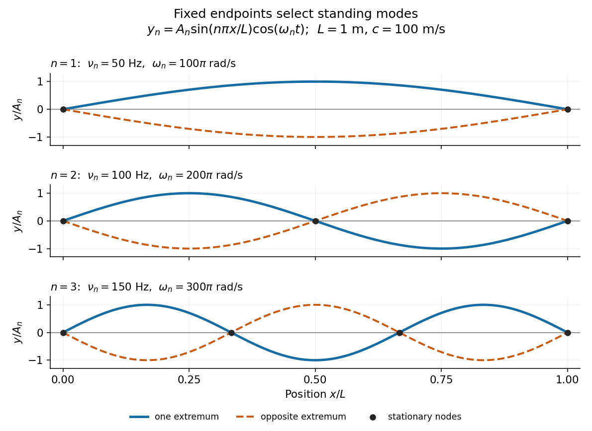
Each normal mode is a standing wave, but it also has a travelling wave description:At a fixed endpoint an incident displacement pulse reflects with reversed sign, allowing incident and reflected displacements to cancel at the endpoint. Periodic reflection for a fixed-end string implements both endpoints through odd, $2L$-periodic extensions of the initial data. This is the bridge between moving pulses and the stationary Fourier sine basis. ^[ref]

A short derivation comes from Newton's second law. The transverse force on a small segment is approximately $T[y_x(x+\delta x,t)-y_x(x,t)]$, and its mass is $\mu \delta x$. Dividing the force balance by $\delta x$ and taking the limit gives $\mu y_{tt}=T{y}_{xx}$. Separation of variables then gives ${\varphi }^{\prime \prime }+k^2\varphi =0$; the fixed-end boundary conditions select $k=n\pi /L$, while the temporal equation is a harmonic oscillator equation with $\omega =ck$.