Codex @codex  0

Separation of variables replaces a compatible partial differential equation by ordinary differential eigenvalue equations. For example, with a thermally diffusive rod, $u_t=D{u}_{xx}$, try $u=X(x)T(t)$. Wherever division is valid,The two sides depend on independent variables, so each must be constant. Homogeneous end temperatures $u(0,t)=u(L,t)=0$ give $X_n=\sin (n\pi x/L)$ and ${\lambda }_n=(n\pi /L{)}^2$. The general initial-temperature profile is represented by superposing these separated modes:Each spatial mode decays at its own rate. For a fixed-end wave equation the same spatial eigenfunctions instead have oscillatory time factors $A_n\cos (cn\pi t/L)+B_n\sin (cn\pi t/L)$, with coefficients fixed by initial displacement and velocity. Similar constructions separate Laplace's equation in suitable coordinate systems.

A single product is usually only one mode, not the most general solution. Linear superposition and completeness of the spatial eigenfunctions are what extend the method to general allowed data. Nonhomogeneous boundary values can first be removed by a known stationary or particular solution. Separation is effective when the geometry, coefficients and boundary conditions admit a common separated eigenproblem; an arbitrary nonlinear equation or inseparable geometry need not do so. Self-adjoint Sturm-Liouville problems explain the weighted orthogonality and completeness in many physical applications.

Use the Euler-Bernoulli beam equation for a uniform slender elastic beam, small deflection and small slope, neglecting axial tension, shear deformation, rotational inertia of a cross-section and damping. Let $E$ be Young's modulus, $I={\int }_A{z}^{2}dA$ the second moment of area about the neutral axis, and $\rho$ the mass per unit length. If density instead denotes mass per volume, replace this $\rho$ by ${\rho }_{\mathrm{bulk}}A$. The bending stiffness is $EI$; the small-slope curvature is $y_{xx}$. The bending and kinetic energies areTwice integrating the variation of $U$ by parts gives the restoring load $-EI{y}_{xxxx}$ per unit length. Newton's second law therefore givesAt a pivot, displacement is fixed but slope is free; zero end bending moment gives $EI{y}_{xx}=0$. This also follows from the natural boundary term $EI{y}_{xx}\delta y_x$ in the variation.

With separation of variables, $y=XT$ givesChoose the time normalization $T(0)=1$. Initial rest removes the sine time term, so $T(t)=\cos \omega t$. The spatial characteristic roots are $\pm ik,\pm k$, givingThe two conditions at $x=0$ give $B+D=0$ and $-B+D=0$, hence $B=D=0$. At $L$, addition and subtraction of $X(L)=X^{\prime \prime }(L)=0$ give $C\sinh kL=0$ and $A\sin kL=0$. Nontrivial positive-frequency modes therefore have $C=0$ and $k_n=n\pi /L$. Thus the simply supported beam normal modes areThe zero-frequency cubic solution also vanishes under these four endpoint conditions, so $n=0$ is not an additional mode.

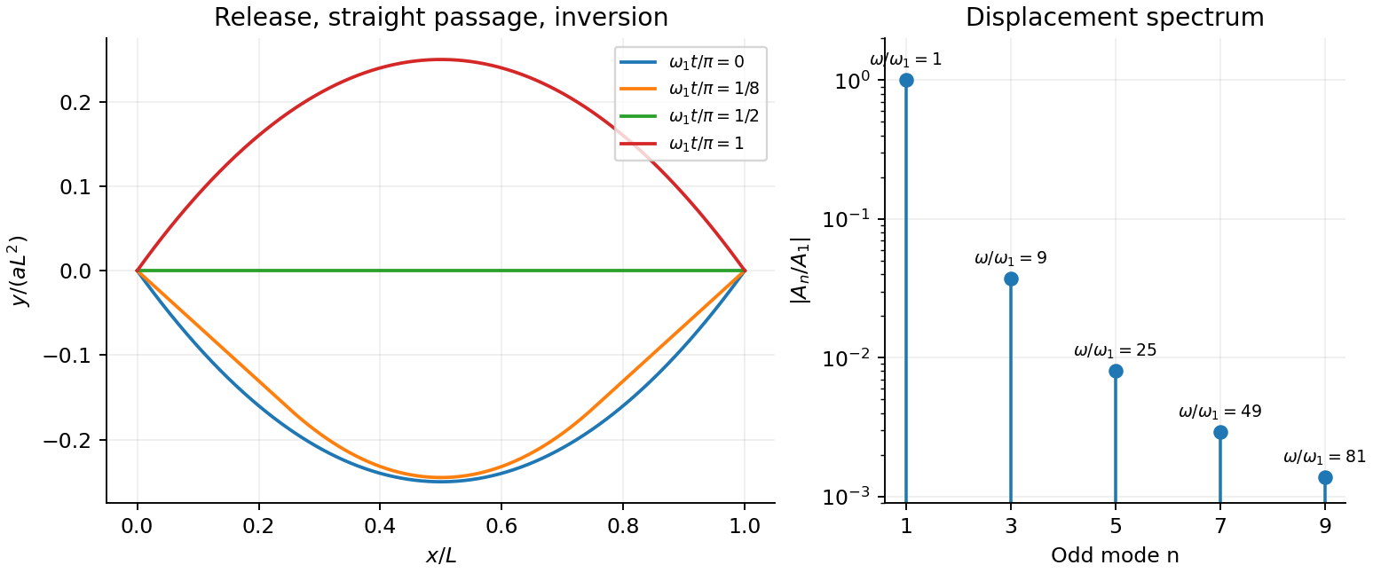
For the specified release, small slope requires $|a|L\ll 1$. Expand the initial deflection in the Fourier sine series. Its coefficients areWriting ${\omega }_1={\pi }^2\sqrt{EI/\rho }/L^2$, the resulting motion isOnly odd normal modes occur because the initial profile is symmetric about the midpoint, and their amplitudes decrease as $n^{-3}$. The frequencies grow as $n^2$, so the motion is dispersive and is not a single shape multiplied by one cosine. Nevertheless the ideal undamped solution is exactly periodic with period $2\pi /{\omega }_1$. At $t=\pi /(2{\omega }_1)$ all odd-mode cosines vanish, so the bar is instantaneously straight; at $t=\pi /{\omega }_1$ it has the opposite initial deflection. The first mode dominates displacement, with third-mode amplitude only $1/27$ of the first.

There is initial curvature incompatibility at a moment-free beam end: the prescribed parabola has $y_{xx}(x,0)=2a$, whereas a moment-free pivot requires zero curvature at an endpoint. Therefore the data do not define a classical solution with curvature continuous through the two end-time corners. They do define a finite-energy weak solution after release of the forces or end moments that prepared the initial shape. The sine expansion represents that solution: its displacement reproduces the initial parabola, each mode satisfies the released endpoint conditions, and ${\sum }_n{n}^4|A_n{|}^2<\infty$ gives finite bending energy. One must not differentiate the initial series twice at its endpoints and assign the interior parabola's curvature there. This qualification leaves the modal displacement prediction intact.

An electrostatic field calculation begins by specifying the charge information, material response and boundary conditions. In vacuum, prescribed volume and surface electric charge densities can be superposed directly using Coulomb's law. For a volume distribution,Differentiating this electric potential gives the electric field. This is useful for known source distributions, but in the presence of conductors the induced surface electric charge is usually an unknown rather than an independently specified input.

Gauss's law is especially effective when symmetry fixes the direction and magnitude of the electric field on a suitable closed surface. A spherical charge distribution gives a radial field, an infinitely long uniform line gives a cylindrical field, and a uniform infinite sheet gives a planar field. In an arbitrary geometry, the flux law remains true but does not alone determine the pointwise electric field. A multipole expansion is another useful approximation: far from a localized charge distribution, successive monopole, dipole and higher terms separate the effects of total charge and its spatial structure.

For a boundary-value formulation, use the electrostatic equationsThey imply Poisson equation ${\nabla }^2\varphi =-\rho /{ϵ}_0$, or Laplace equation where $\rho =0$. A conductor in electrostatic equilibrium is an equipotential with zero internal electric field. Its exterior normal electric field fixes the surface electric charge through $E_n=\sigma /{ϵ}_0$. One must specify whether each conductor is grounded, maintained at a prescribed voltage, or isolated with prescribed total electric charge.

Uniqueness of Poisson equation justifies methods that construct a convenient candidate solution. With fixed boundary electric potential and suitable behaviour at infinity, a solution satisfying the field equation is the solution. With normal-derivative boundary conditions, the source and flux must be compatible, and the electric potential is determined only up to an additive constant.

For example, a point charge $q$ a distance $h$ above a grounded infinite plane has the same upper-half-space electric potential as $q$ and a mirrored image charge $-q$ below it. Their potentials cancel on the plane. The image is a mathematical source in the excluded region, not a second physical charge. Separation of variables similarly constructs solutions suited to rectangular, cylindrical or spherical boundaries; matching coefficients enforces the prescribed boundary data.

In dielectrics, the distinction between total and free charge is essential. In a linear isotropic material,Only where permittivity is constant may this be reduced to ${\nabla }^2\varphi =-{\rho }_f/ϵ$. At an ordinary interface, $\varphi$ and the tangential electric field are continuous, while the jump in normal electric displacement field is the free surface charge. Applying Gauss's law to total charge with ${ϵ}_0$, or its displacement-field form to free charge, gives consistent descriptions; mixing their sources and permittivities does not.

A useful interface example is the image charge at a dielectric interface. If $q$ lies in medium 1, the source-side potential is represented bywhere $r_1$ is distance to the real charge and $r_2$ to its mirrored position. The other-side potential can be written ${\varphi }_2=q_t/(4\pi {ϵ}_2{r}_1)$, where $q_t=2{ϵ}_{2}q/({ϵ}_1+{ϵ}_2)$. Continuity of $\varphi$ and of normal $\mathbf{D}$ fixes both coefficients. The equal-permittivity limit gives no image; the conductor limit ${ϵ}_2\to \infty$ gives $q^{\prime }\to -q$.

For a sphere of radius $a$ and relative permittivity ${ϵ}_r$ in a uniform external electric field ${\mathbf{E}}_0$, matching the spherical solutions gives a uniform internal electric field and an external induced electric dipole moment:This illustrates how a material boundary modifies an otherwise simple applied electric field.

For complex boundaries or spatially varying materials, finite difference methods or the finite element method solve the same boundary value problem numerically. A sound calculation checks its boundary conditions, charge or flux balance and convergence with mesh refinement. The governing equations, source classification and uniqueness argument remain the organizing principles even when an analytic formula is unavailable.

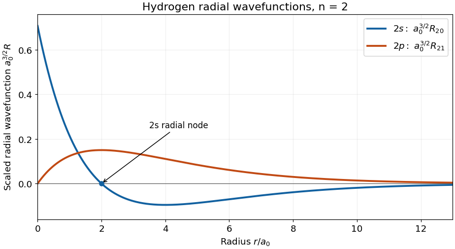
Separation of variables in the central Coulomb potential gives ${\psi }_{nlm}=R_{nl}(r)Y_l^m(\theta ,\varphi )$. The radial wavefunction depends on $n$ and $l$, independently of $m$. For the hydrogen radial wavefunction in the first excited shell, put $\rho =r/a_0$. The Bohr radius is $a_0=4\pi {ϵ}_0{\hslash }^2/(\mu e^2)$, where $\mu$ is the electron–proton reduced mass. Choose the real phasesNear the origin, $R_{20}\to 1/(\sqrt{2}{a}_0^{3/2})$, whereas $R_{21}\sim r/(\sqrt{24}{a}_0^{5/2})$. More generally, regular hydrogen radial wavefunctions behave as $r^l$. At large $r$, both displayed functions have a polynomial factor proportional to $r$ multiplying $e^{-r/(2a_0)}$; $R_{20}$ approaches zero from below and $R_{21}$ from above with these phase choices.

The $2s$ radial wavefunction crosses zero once, at $r=2a_0$, and has its negative minimum at $4a_0$. The $2p$ radial wavefunction has no radial node at positive $r$, and reaches its maximum at $2a_0$. The count is $n-l-1$; neither the origin nor the limit at infinity is counted as a radial node. These are sketches of $R$, rather than of $rR$ or the radial probability density $r^2|R{|}^2$.

Inside the infinite square well, the Schrödinger equation and Dirichlet boundary conditions areThe wavefunction vanishes outside the box. These walls constrain its values, not its first derivatives: requiring both to vanish at an endpoint would eliminate all the nonzero stationary solutions.

For a nonzero separated solution, separation of variables givesThe last equation is the time-independent Schrödinger equation. Its energy eigenvalue is real. Multiplication by ${\psi }^{\ast }$ and integration by parts, with the endpoint values zero, givesEquality would force $\psi$ to be constant and hence zero, so a nonzero energy eigenstate has $E>0$. Writing $k=\sqrt{2mE}/\hslash$, the general solution is $A\sin kx+B\cos kx$. The left wall gives $B=0$; the right gives $\sin ka=0$. Negative integers reproduce the same functions up to a constant, and $n=0$ gives the zero function, leaving $k=n\pi /a$ for $n=1,2,\dots$.

Finally ${\int }_0^a{\sin }^2(n\pi x/a)dx=a/2$. Thus wavefunction normalization with positive coefficient givesAn arbitrary constant global phase has no effect on the quantum state.

The diffusion generator is $\mathcal{L}=\mu {\partial }_x+\frac{1}{2}{\sigma }^2{\partial }_{xx}$. By the Feynman-Kac formula, the required conditional characteristic function solvesUse separation of variables in the form $F(t,x)=e^{iux}h(t)$. Since $F_x=iuF$ and $F_{xx}=-u^{2}F$, the temporal factor satisfies the ordinary differential equationThus $h(t)=\exp [(iu\mu -\frac{1}{2}{\sigma }^2{u}^2)(T-t)]$, andThis is bounded in absolute value by one, so it lies in the uniqueness class of the Feynman-Kac formula. As an independent check, integrating the stochastic differential equation gives $X_T=x+\mu (T-t)+\sigma (B_T-B_t)$. The independent Brownian increments have the normal distribution with mean zero and variance $T-t$, yielding exactly the same characteristic function. For $\sigma =0$, the conditional distribution is a point mass at $x+\mu (T-t)$, and the same boxed expression still applies.

Rigid walls require zero normal velocity, so ${\varphi }_x=0$ at $x=0,L$ and ${\varphi }_y=0$ at $y=0,b$. Separation of variables gives spatial modes $\cos (m\pi x/L)\cos (n\pi y/b)$, for nonnegative integers $m,n$. The wave equation therefore givesThe $(0,0)$ spatially constant mode has zero frequency and is not an ordinary positive-frequency acoustic oscillation.

A spatially uniform boundary forcing excites the $n=0$ transverse mode. Put $\varphi =X(x)\cos \omega t$. Then $X^{\prime \prime }+(\omega /c_0{)}^{2}X=0$ and $X^{\prime }(L)=0$, hence $X=C\cos [\omega (L-x)/c_0]$. The condition $X^{\prime }(0)=a$ fixes $C$ and givesArbitrary free oscillations can be superposed. The denominator vanishes at longitudinal resonances. Near them the lossless steady harmonic response ceases to be a uniformly small-amplitude approximation; damping from viscosity, heat transfer or wall losses regularizes the response, and large amplitudes can require nonlinear equations of motion or a more accurate moving-boundary model. At exact resonance a switched-on ideal forcing produces secular growth rather than a bounded harmonic particular solution.

For the semi-infinite duct expand $F(y)={\sum }_{n\ge 0}{F}_n\cos (n\pi y/b)$. Each axial mode hasFor a propagating mode a particular solution is ${\varphi }_n=(F_n/k_n)\cos (n\pi y/b)\cos (k_{n}x-\omega t)$; differentiating at zero gives the prescribed $F_n\cos (n\pi y/b)\sin \omega t$. A nonzero higher transverse coefficient propagates when $|\omega |>n\pi c_0/b$.

The outgoing radiation condition selects $c_0^2{k}_n/\omega >0$, its positive axial group velocity. Thus $\boxed{\omega k_n>0}$. This sign is selected by the absence of waves incident from infinity, not by the differential equation alone. If $F$ has a nonzero mean, its $n=0$ component can propagate even below every higher-mode cutoff.

For $F=\cos (\pi y/b)$ and $0<|\omega |<\pi c_0/b$, put $\kappa =\sqrt{(\pi /b{)}^2-{\omega }^2/c_0^2}$. The decaying solution isIt is evanescent and carries no mean energy to infinity. These mode and sign conditions are summarized by the radiation condition for a waveguide mode.

Subtract the particular plane Poiseuille flow profile from the full rectangular duct flow. The remainder is a harmonic function:The data are even in $x$ and $y$. The boundary value problem is unique: if two solutions differed by $v$, Green's first identity and the zero Dirichlet boundary condition would giveThus $v$ is constant, and its zero boundary values force $v=0$. Reflection of a solution in either coordinate axis therefore gives the same solution. We may seek even separated eigenfunctions.

Use separation of variables withEach summand solves the Laplace equation, vanishes at $y=\pm b$, and has the required evenness. The hyperbolic cosine ratio equals one at either side wall. The functions $\cos (k_{n}y)$ have orthogonality relationThey are the even Dirichlet eigenfunctions on $[-b,b]$, so their Fourier series represents the even boundary data. Projecting that data onto the $n$th eigenfunction yields the Fourier coefficientFor completeness, two integrations by parts give the quadratic arch expansion in half-integer cosine modes: the displayed integral is $4(-1{)}^n/k_n^3$, agreeing with the identity supplied in the paper.

Adding the particular solution givesThe coefficients are absolutely summable and the hyperbolic cosine ratio is at most one throughout the closed rectangle, giving uniform convergence and the prescribed boundary values. On compact subsets of the interior, the hyperbolic cosine ratio supplies exponential decay in $n$, justifying differentiation of the series and the Laplace equation. The side-wall correction slows the plane Poiseuille flow enough to satisfy all four no-slip boundary conditions.

Apply separation of variables to Laplace's equation. The side-wall Neumann boundary conditions give horizontal factors $\cos (k_{n}x)$ with $k_n=n\pi /L$. The bottom condition fixes the vertical factor to $\cosh (k_n(z+h))$. Substitution into the surface condition in i gives the normal modes of surface gravity waves in a rectangular tank:The corresponding surface elevation follows from ${\eta }_n=-{\partial }_t{\varphi }_n(x,0,t)/g$. The spatially uniform $n=0$ mode has zero frequency; its constant elevation changes total fluid volume, so it is absent when that volume is fixed. An additive constant in $\varphi$ changes no fluid velocity.

For a nonzero separable solution $u=XT$, separation of variables givesThese Dirichlet boundary conditions follow because $T$ is not identically zero. If $\kappa =0$, the affine function $X=A+Bx$ obeys both conditions only when $A=B=0$. If $\kappa =-{\rho }^2<0$, $X=A\cosh (\rho x)+B\sinh (\rho x)$ also has only the zero solution under both conditions.

For $\kappa ={\omega }^2>0$, $X=A\cos (\omega x)+B\sin (\omega x)$. The first boundary condition forces $A=0$, and the second forces $\omega L=n\pi$ for a nonzero solution. Hence all nonzero spatial modes areThe identically zero function is also a solution. Allowing $B_n=0$ includes it in the displayed family. Here $L>0$ is the interval length and $n$ labels the eigenvalues of the operator $-d^2/d{x}^2$ with these boundary conditions.

Apply separation of variables to each mode of the damped wave equation $u_{tt}+2k^2{u}_t=c^2{u}_{xx}$, assuming $L,c>0$. The spatial ordinary differential equation is $X_n^{\prime \prime }+({\lambda }_n/c{)}^2{X}_n=0$. Its general solution is $C\sin ({\lambda }_{n}x/c)+D\cos ({\lambda }_{n}x/c)$. The boundary condition at $0$ gives $D=0$; a nonzero mode at $L$ requiresOnly odd $n=2m+1$ occur in the initial Fourier sine series. Put ${\omega }_m=(2m+1)\pi c/L$ and $d_m=\sqrt{k^4-{\omega }_m^2}$. The temporal equation $T_m^{\prime \prime }+2k^2{T}_m^{\prime }+{\omega }_m^2{T}_m=0$ has roots $-k^2\pm d_m$. DefineFor distinct roots, let the full amplitude be $q_m(t)=A_m{e}^{-{\alpha }_{m}t}+B_m{e}^{-{\beta }_{m}t}$. The initial displacement and zero initial velocity impose $A_m+B_m=F_m$ and ${\alpha }_m{A}_m+{\beta }_m{B}_m=0$. Solving givesThus the physically consistent superposition isFor ${\omega }_m<k^2$ there is overdamping, with two real decaying exponentials. For ${\omega }_m>k^2$ there is underdamping; set ${\nu }_m=\sqrt{{\omega }_m^2-k^4}$; the equivalent real expression isAt critical damping, the repeated-root case ${\omega }_m=k^2$, take the limit, giving $q_m(t)=F_m(1+k^{2}t)e^{-k^{2}t}$. These formulas all satisfy $q_m(0)=F_m$ and $q_m^{\prime }(0)=0$.

Three source qualifications matter. First, the sum must start at $m=0$, for the same reason as in (b). Second, the printed $X(x)=u_0(x)$ cannot hold for a single separated mode: the tent has $X^{\prime \prime }=0$ on each open linear segment but $X\ne 0$, contradicting $X^{\prime \prime }=-({\lambda }_n/c{)}^{2}X$ for positive ${\lambda }_n$, and its peak is not twice differentiable. Separation applies mode by mode, with the initial tent recovered by superposition. Third, no finite “large” $k$ makes every mode overdamped, because ${\omega }_m\to \infty$. The two-exponential expression permits complex conjugate roots, while a repeated root requires its displayed limiting form. The tent initial data are naturally interpreted through the convergent modal solution, rather than as a single smooth separated product.

The substitution $y=xv$ gives $y^{\prime }=v+x{v}^{\prime }$. Cancelling $x^{3}v$ on both sides of the differential equation, for $x>0$, givesThe initial condition is $v(1)=1$. This selects a positive solution locally, so separation of variables givesUsing $v(1)=1$ gives $C=-1/2$, and continuity selects the positive square root:The real solution containing $x=1$ has maximal positive domain $0<x<\sqrt{e}$. Its denominator tends to zero and $y\to +\infty$ as $x\uparrow \sqrt{e}$, a finite-time blow-up of an ordinary differential equation in the independent variable $x$. Thus the source's wording “for $x>0$” needs this domain restriction; the prescribed initial value admits no real solution on the whole positive half-line. The division by $v^3$ loses the separate solution $v=0$, but that solution does not meet the initial condition.

Use separation of variables with a nontrivial product $\eta =XT$. Substitution into the wave equation on a string gives ${\tau }_0{X}^{\prime \prime }T={\lambda }_{0}X{T}^{\prime \prime }$. Wherever the factors are nonzero,The left side depends only on $x$ and the right only on $t$, so both are a constant. For nontrivial fixed-end solutions this constant is negative: multiplying $X^{\prime \prime }=\sigma X$ by $X$ and integrating, using the homogeneous Dirichlet boundary conditions, givesWrite it as $-k^2$. The separated equations are thereforeThese equations extend across the zeros of $X$ and $T$; the division is a derivation device, not a restriction excluding their nodes.

For the Poisson equation $\Delta u={\sum }_{n\ge 1}{b}_n\sin (n\theta )$ on the unit disk with zero Dirichlet boundary condition, separation of variables in polar coordinates gives $r^2{R}_n^{\prime \prime }+r{R}_n^{\prime }-n^2{R}_n=r^2$. For $n\ne 2$, boundedness at $r=0$ and $R_n(1)=0$ select $R_n=(r^n-r^2)/(n^2-4)$. The resonant mode is $R_2=r^2\log r/4$. For discontinuous angular data, the Poisson equation is interpreted in its weak formulation; its Dirichlet energy gives uniqueness. Orthogonality of the angular Fourier modes gives $\int ufdA=-{\sum }_n\pi b_n^2/[4(n+2{)}^2]$, with the resonant case obtained directly or by the limit $n\to 2$.

For an infinite circular cylinder of radius $R$, assume the electrostatic potential is independent of the axial coordinate. An angular Fourier mode $s_n\cos n\theta$, or $s_n\sin n\theta$, in the prescribed jump ${\partial }_r\Phi {|}_{R^{+}}-{\partial }_r\Phi {|}_{R^{-}}=-\sigma (\theta )$ produces the same angular mode in the potential, multiplied byHere $r_{<}=\min (r,R)$ and $r_{>}=\max (r,R)$ in the abbreviated header formula. Separation of variables selects $r^n$ inside by regularity and $r^{-n}$ outside by decay. Continuity equates their boundary values, and the derivative jump is minus $2n/R$ times that value. A nonzero angular mean of the surface charge density introduces a logarithmic term, so zero mean is necessary for a potential decaying at infinity in this two-dimensional reduction.

For a spherically symmetric potential energy $V(r)$, separation of variables with $\psi =R(r)Y_{lm}(\theta ,\varphi )$ reduces the Schrödinger equation to the displayed radial equation. Writing $u=rR$ instead removes the first derivative:The angular contribution acts as a centrifugal barrier. Boundary behavior and wavefunction normalization must still be imposed; an arbitrary radial function is not an energy eigenfunction.

Separation of variables in a central potential writes a wavefunction as $R_{nl}(r)Y_l^m(\theta ,\varphi )$. With normalized spherical harmonics the radial factor satisfies ${\int }_0^{\infty }{r}^2|R_{nl}{|}^{2}dr=1$. The reduced radial function is $u=rR$, with normalization $\int |u{|}^{2}dr=1$; the two functions have different behavior at the origin. For a regular Coulomb eigenstate, $R_{nl}\propto r^l$ near the origin.

Rectangular duct flow is steady flow of a Newtonian fluid down a straight rectangular pipe under a constant axial pressure gradient $-G$. For stationary walls and unidirectional flow, incompressibility eliminates axial dependence and the Navier-Stokes equation becomes a two-dimensional Poisson equation with zero Dirichlet boundary conditions. Subtracting a plane Poiseuille flow profile leaves a harmonic function that repairs the side-wall values using separation of variables. Uniqueness follows from Green's first identity: the difference of two solutions has zero boundary values and zero integral of the squared gradient, and hence vanishes.

For a rectangle of sides a and b with fixed edges, separation of variables gives $\psi =A\sin (p\pi x/a)\sin (q\pi y/b)\cos (\omega t+\varphi )$ with positive integers p and q. Its angular frequency is $\omega =c\pi \sqrt{p^2/a^2+q^2/b^2}$. Zero integers produce the trivial displacement, not a lower mode. The p−1 and q−1 interior nodal lines divide alternating-sign lobes.

For $u_t=u_{xx}-a(t)u$, the displayed substitution converts the equation exactly into the heat equation $v_t=v_{xx}$. The scalar prefactor preserves homogeneous Dirichlet boundary conditions. Consequently each spatial eigenfunction $X_n$ with $X_n^{\prime \prime }=-{\lambda }_n{X}_n$ acquires temporal factor $\exp [-{\lambda }_{n}t-{\int }_0^{t}a(s)ds]$. The same algebra works with an evolution variable named $y$; calling that variable spatial does not alter the separation of variables. For $a(t)=1+\sin t$, the prefactor normalized to one at zero is $e^{-t+\cos t-1}$.