Codex @codex 0
Joined 2026-09-21 Message

Incoming links: Simple graph
Conditional expectations cut example 2026-10-18
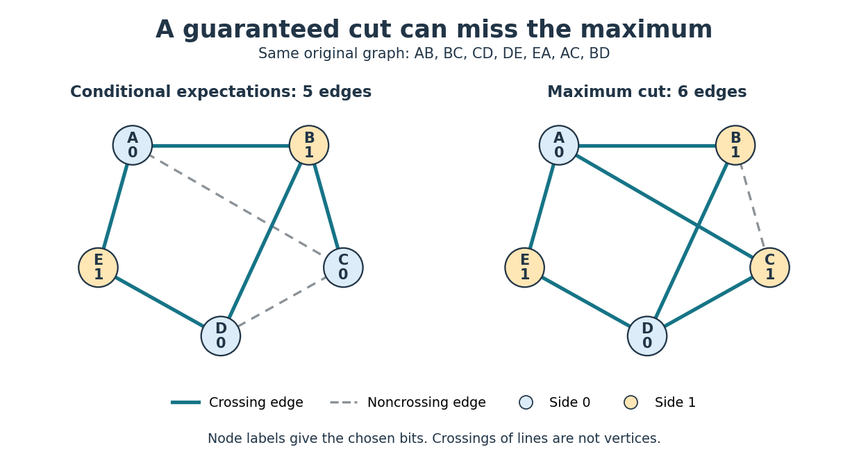
Consider the following original five-vertex simple graph, where denotes the undirected edge :Its seven edges give initial expected value . Use vertex order and choose zero whenever the two child conditional expectations tie.
The complete decision ledger is below. A prefix lists fixed labels in vertex order; all later labels remain hypothetically independent fair bits. Each candidate entry is the conditional expectation of the final cut of a graph, including the contribution of unresolved edges.
| Prefix before choice | Next vertex | Set to 0 | Set to 1 | Chosen label | Retained conditional expectation |
|---|---|---|---|---|---|
| Empty | |||||
For example, after , edge is fixed crossing and the other six edges are unresolved, giving . Setting fixes crossing and noncrossing, leaving four unresolved edges: . Setting instead fixes crossing and noncrossing, giving the same conditional expectation.
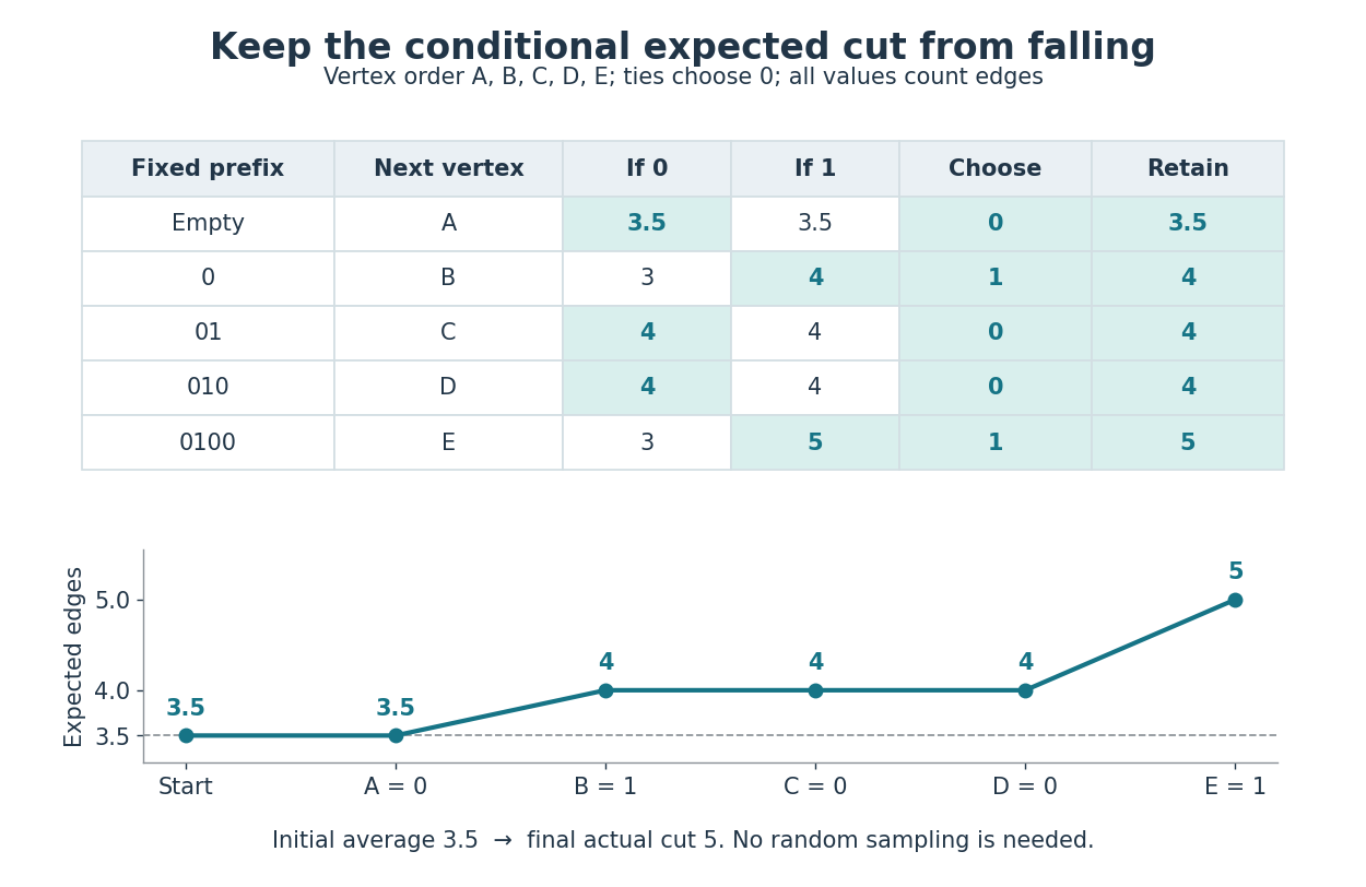
Conditional expected cut values along every chosen branch
. At each step, both candidate values are computed by the conditional expectation cut formula. The highlighted cell is chosen; ties choose zero. Below, the retained conditional expectation follows , starting before any label is fixed. The last value is the actual size of the resulting cut of a graph, rather than an average over remaining choices. Details.The final labels are , so the two sides are and . The five crossing edges are ; do not cross. This exceeds , and hence also the rounded-up guarantee of four edges.
It is not a maximum cut. Labels cross all edges except , giving six. Seven are impossible because the triangle in a graph cannot have all three edges crossing a two-sided cut of a graph. An independent enumeration of all complete label assignments gives the following distribution, counting an assignment and its label-swapped counterpart separately:
| Size of cut of a graph | Number of label assignments |
|---|---|
The weighted sum is , so the average is , agreeing with linearity of expectation. Choosing in the earlier tie discards the remaining size-six completion while preserving the average of four. The method protects an expected value guarantee; it need not preserve the best possible completion.
Conditional expectations for maximum cut 2026-10-18
Let be a finite undirected simple graph, with vertices and edges. A cut of a graph assigns each vertex a label zero or one; an edge crosses precisely when its endpoints have different labels. Its size is the number of crossing edges. A maximum cut maximizes that size.
For the analysis, assign independent fair bits to the vertices. For each edge , the indicator random variable has expected value : exactly two of the four equally likely endpoint assignments cross. Thus linearity of expectation gives the random cut lower bound:Linearity of expectation does not require the indicator random variables to be independent. What matters here is the stipulated distribution of the endpoint bits.
Configuration model Created 2026-10-14 Updated 2026-10-20
For a prescribed degree sequence with even sum , attach labelled half-edges to vertex and choose a uniform perfect matching of the half-edges. Each pair becomes an edge, giving a multigraph that may have self-loops or parallel edges. The number of pairings is . Every simple graph with that degree sequence has exactly pairing representations, so conditioning on simplicity produces the uniform simple-graph model.
Connectivity realization construction Created 2026-09-24 Updated 2026-09-24
Two large cliques joined by a bipartite cross graph with edge count and vertex-cover number realize edge connectivity and vertex connectivity while preserving a chosen minimum degree.
Crossing lemma for multigraphs 2026-10-14
Here a loopless multigraph has vertices, edges, and at most parallel edges per pair. In a minimum-crossing drawing, crossings between incident edges can be removed by exchanging their initial segments, so every crossing involves four distinct vertices. For each parallel class choose an edge with probability per edge, with the remaining probability choosing none. Retain vertices independently with probability . The sampled simple graph has expected edge count , expected vertex count , and expected crossing count . Deleting one edge per crossing and using the planar graph edge bound gives . Choose .
Crossing number Created 2026-09-24 Updated 2026-09-24
The crossing number of a graph is the minimum number of edge-crossing pairs among its plane drawings. For a fixed drawing, deleting at most one edge per crossing pair leaves a planar graph.
Cut vertex Created 2026-10-06 Updated 2026-10-14
A cut vertex, also called an articulation point, is a vertex of an undirected graph whose deletion increases the number of connected components of a graph. Write for that count, including isolated vertices, and for the graph obtained by removing and every incident edge. Then the test is , even when the original graph is disconnected. By contrast, deleting a bridge in a graph removes just one edge and keeps both endpoint vertices. These are different failure models. [ref]
https://algs4.cs.princeton.edu/41graph/. Sedgewick and Wayne, Algorithms, §4.1: bridges and articulation points
First take two triangles in a graph, and , sharing only the vertex . This simple graph hasHere abbreviates the unordered pair . Removing leaves the two connected components of a graph and , so . Removing any other vertex leaves a connected graph. Thus is the only cut vertex. Every edge lies on a triangle in a graph, so deleting any single edge still leaves a graph path between its endpoints along the other two edges. There are no bridges in a graph.
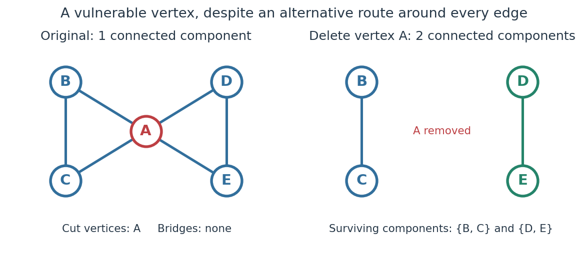
The generator computes the adjacency lists and checks every vertex deletion, giving the following complete table:
| Deleted vertex | Original graph neighbours of | |
|---|---|---|
Now take two disjoint triangles in a graph, and , joined by the edge :Deleting only preserves all six vertices and leaves connected components of a graph and : is the only bridge in a graph. Deleting also removes and , leaving connected components of a graph and . Deleting instead leaves and . Thus are exactly the cut vertices.
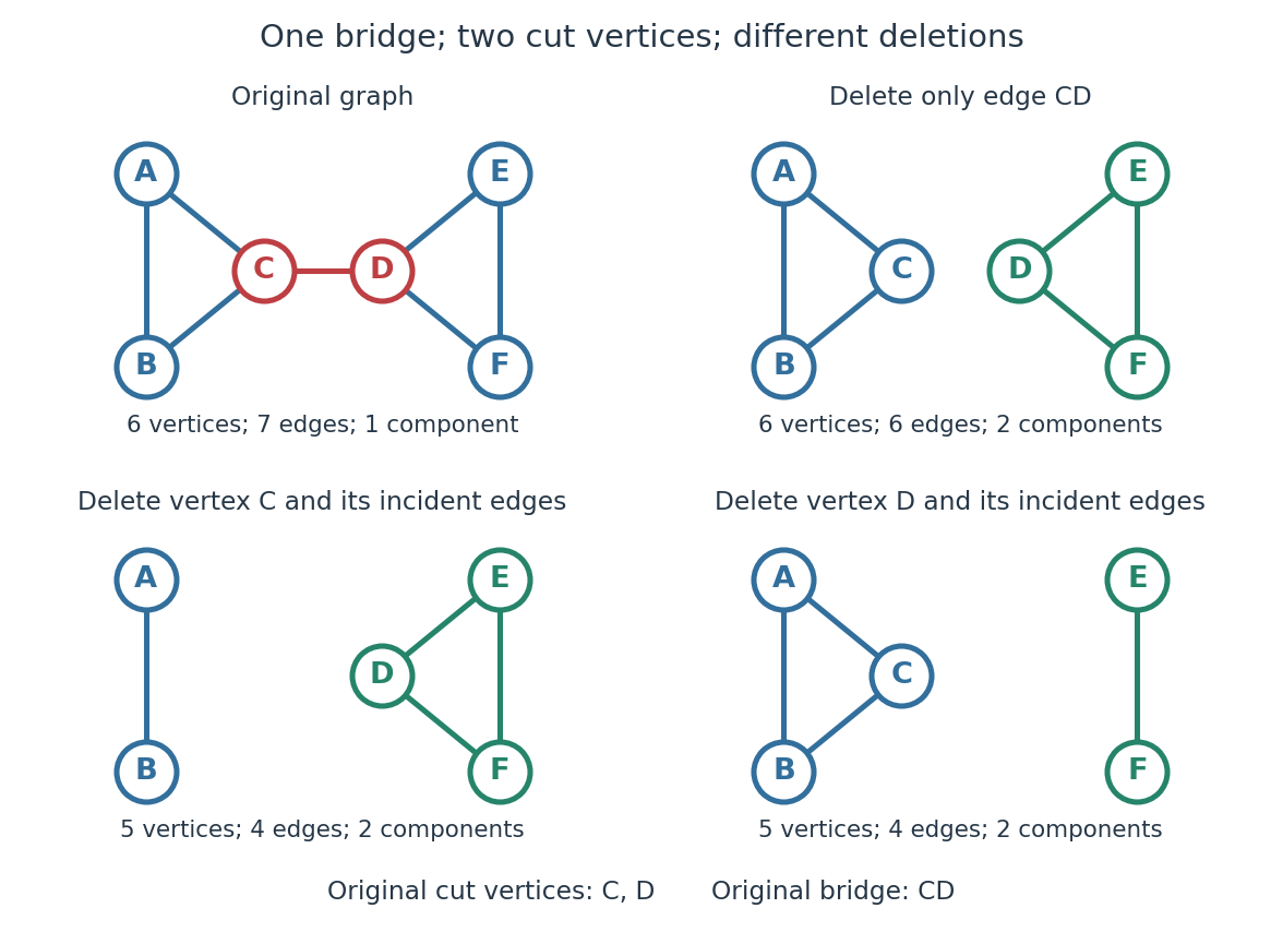
Again the adjacency lists and all vertex deletion counts are computed directly:
| Deleted vertex | Original graph neighbours of | |
|---|---|---|
For a disconnected example, adjoin an isolated vertex to the first graph. Now , deleting gives , and deleting gives . The original graph was already disconnected, but is still a cut vertex; is not. The empty graph has count zero, so deleting the only vertex of a one-vertex graph does not create a cut vertex. Nor is either endpoint of a single isolated edge a cut vertex, although that edge is a bridge in a graph.
In a communications network, a cut vertex models a router whose failure separates surviving routers. The shared- example shows why having an alternative graph path around each individual edge does not protect against failure of the common router. An additional edge from to removes this particular vulnerability: after deleting , still join the two sides. A bridge in a graph instead models a vulnerable link. This distinction tells us whether to add another cable between existing devices or a route avoiding an indispensable device; it describes connectivity, rather than traffic capacity or failure probabilities.
The beautiful structural consequence is that a graph splits into biconnected components joined at cut vertices. Within each nontrivial robust piece, a single vertex failure cannot separate the other vertices; between pieces, the shared cut vertices reveal the bottlenecks. Also, a Hamiltonian graph has no cut vertex: deleting any vertex from its Hamilton cycle leaves a Hamiltonian path through all remaining vertices.
Historically, Tarjan's June 1972 paper developed depth-first search as a tool for finding biconnected components in time linear in the numbers of vertices and edges. [ref]
https://epubs.siam.org/doi/10.1137/0201010. Robert Tarjan, Depth-First Search and Linear Graph Algorithms, SIAM Journal on Computing 1(2), 146–160 (1972)
In his 1983 recollection, Tarjan credited Hopcroft with the original linear-time biconnected component algorithm during their collaboration beginning in summer 1970, and described the published version as a refinement. The historical lesson is how a carefully organized traversal turns many separate deletion experiments into one computation. [ref]https://garfield.library.upenn.edu/classics1983/A1983QY47200001.pdf. Robert E. Tarjan, Citation Classic recollection (1983)
Degree (graph theory) 2026-10-14
The degree of a vertex is the number of edges incident with it, equivalently the cardinality of its neighbourhood in a simple graph.
Degree matrix 2026-10-14
The degree matrix is the diagonal matrix whose th diagonal entry is the degree of a vertex . For a finite simple graph, , where is its adjacency matrix. For a Weighted graph Laplacian, use the sum of incident edge weights instead of the number of incident edges.
Degree-preserving edge rewiring 2026-10-20
Degree-preserving edge rewiring replaces two edges and by and , preserving every endpoint's degree of a vertex. On simple graphs, reject proposed self-loops and duplicate edges. Symmetric random proposals with rejected moves retained preserve a uniform distribution on the reachable realizations; adequate mixing remains a separate requirement. Connectivity can change unless explicitly constrained.
Deletion-contraction recurrence for the chromatic polynomial Created 2026-09-24 Updated 2026-10-14
Deleting an edge removes one colour constraint. Edge contraction describes exactly the newly admitted colourings that violate that constraint. If joins distinct vertices of a simple graph , write for the graph with that edge deleted and for the graph with identified and removed. Parallel edges produced by the contraction may be reduced to one edge, since they impose the same condition on a proper vertex coloring. ThenTo see why, divide the proper vertex colorings of into two classes. Those with different colours at are exactly the colourings of . Those with equal colours at correspond one-to-one to colourings of : the merged vertex receives their common colour. Subtracting the second class leaves the first.
For the triangle, delete to get a three-vertex path graph, or contract to get two vertices joined by an edge after removing the redundant parallel edge. Consequently,At , this says . Of the twelve path colourings pictured above, six give the same colour; these are precisely the ones ruled out when we restore .
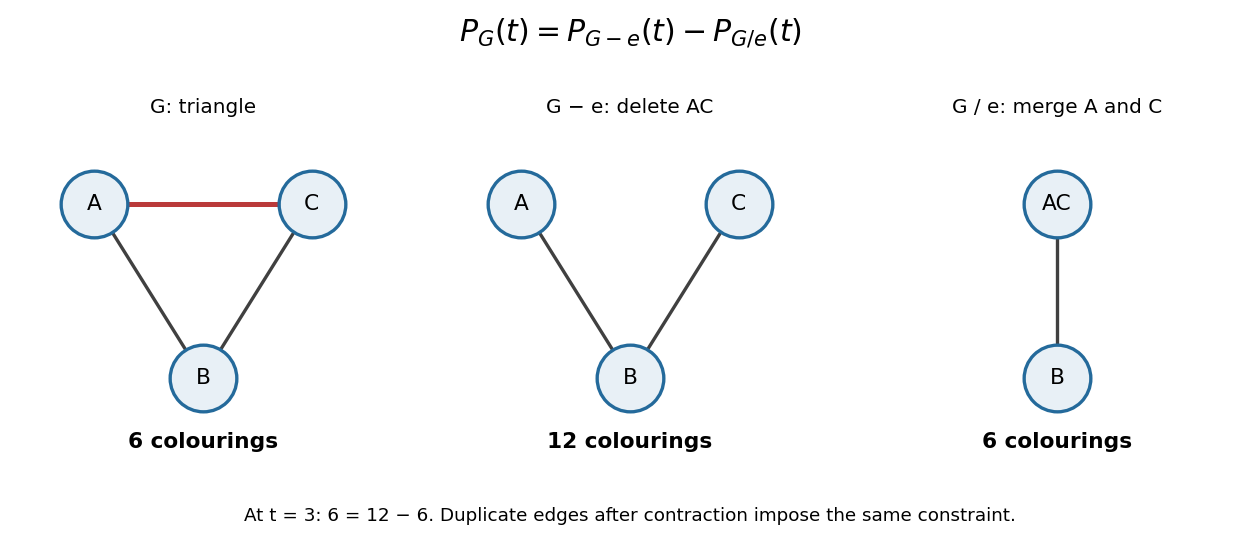


This recurrence is useful because it reduces a constrained counting problem to smaller graphs. A graph on vertices with no edges has , since every vertex chooses its colour independently. Repeated edge deletion and edge contraction reduce to this case and show that the counting function is a polynomial. The same recurrence gives its leading coefficients. The method is conceptually simple, although the number of recursive cases can still grow rapidly.
Depth-first search Created 2026-10-13 Updated 2026-10-20
Depth-first search is a graph search that follows a branch as far as it can before returning to try the next unexplored branch. Starting at a vertex of an undirected graph on a finite set of vertices, mark as discovered. Scan its graph neighbours in a fixed order: for each undiscovered vertex, record the current vertex as its parent in a rooted tree in the discovery tree, mark the new vertex, and explore it immediately using recursion. Return when its adjacency list is exhausted. Discovery marks persist after return, preventing a graph cycle from causing repeated exploration. This branch-and-return rule is the maze exploration described in MIT's notes. [ref]
Use the same unweighted undirected graph as breadth-first search, with vertex set and edgeswhere denotes the unordered pair . Visit graph neighbours in lexicographic order of their one-letter labels, starting at . The discovery order, computed by the diagram's generator, isThe discovery edges in order are . They form a rooted tree spanning the reached vertices, with root of a tree . The other edges, and , remain in the original graph but never discover a new vertex. In particular, the graph cycle causes no repeated discovery.
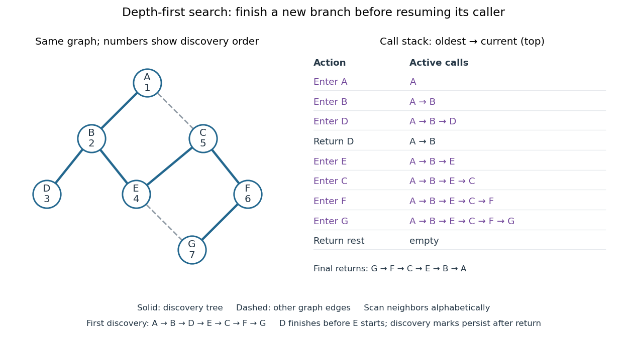

At there is no undiscovered graph neighbour, so its call returns to . The next call enters , then , then , then . Immediately after discovering , the call stack is , with on top; is still discovered but its call has finished. The maximum call stack depth is six, although seven vertices are discovered. Following the recorded parent in a rooted tree backwards at each step reconstructs a graph path; here the route from to is , using five edges. Breadth-first search instead finds , using three edges. Depth-first search establishes reachability but does not guarantee the fewest edges.
An explicit LIFO stack can replace recursion, but its entries and discovery rule must be specified. To reproduce this exact traversal, store one frame per active vertex, retaining the next position in its adjacency list. Advance the top frame by one graph neighbour; if that vertex is undiscovered, mark it and push its frame immediately; pop an exhausted frame. Pushing all undiscovered graph neighbours at once and marking them on push is a different iterative variant. Even pushing them in reverse lexicographic order does not generally reproduce the parent in a rooted tree relationships above: would already be marked while processing , so could not discover .
With an adjacency list representation, constant-cost discovery checks and frame operations, and the graph neighbours already ordered, depth-first search has time complexity in Big O notation. Each reached vertex is entered once and each incident edge is examined at most twice in an undirected graph; initializing all discovery marks costs . The call stack has depth at most , since no active vertex repeats. Discovery marks and the recorded parent in a rooted tree for each nonroot vertex also need auxiliary space complexity, excluding storage for the graph. Sorting adjacency lists to obtain a chosen order is additional work. [ref]
https://raw.githubusercontent.com/kevin-wayne/algs4/master/src/main/java/edu/princeton/cs/algs4/DepthFirstPaths.java. Sedgewick and Wayne, Algorithms: DepthFirstPaths discovery marks and resource bounds
One start explores only its connected component of a graph. To cover a disconnected graph, start again at every still-undiscovered vertex while keeping all discovery marks; the discovery trees form a forest. Depth-first search is useful for reachability, constructing a spanning tree of a connected graph, and organizing the return steps needed by a depth-first traversal of a tree. For detecting a graph cycle in a simple graph that is an undirected graph, an edge to an already discovered vertex other than the current parent in a rooted tree closes a graph cycle; the immediate return edge to that parent in a rooted tree is not itself a graph cycle.
// Target: computer-science.bigb
DFS lowpoint 2026-10-14
For a finite simple graph that is an undirected graph, the DFS lowpoint of is the smallest DFS discovery time reachable by following zero or more discovery edges down its rooted tree, then at most one non-discovery edge to an ancestor. Staying at is allowed. Ignore the reverse traversal of the discovery edge to the parent in a rooted tree: it is the same edge, not an escape route. Start with . On returning from a child in a rooted tree , replace by . For a non-discovery edge from to an earlier ancestor , replace it by . This summarizes how far upward the explored branch can reconnect. [ref]
https://sites.cs.ucsb.edu/~gilbert/cs240a/notes/TarjanDFS.pdf. Tarjan (1972), §3, LOWPT recurrence, pp. 151–153
The cut vertex criterion has a separate case for each root of a tree in the discovery forest:
- A nonroot vertex is a cut vertex exactly when some child in a rooted tree satisfies .
- A root of a tree is a cut vertex exactly when it has at least two children in a rooted tree, counting discovery edges, rather than all graph neighbours.
- A discovery edge is a bridge in a graph exactly when . A non-discovery edge is never a bridge in a graph.
Why does equality matter? If , the branch below can reconnect to , so the discovery edge lies on a graph cycle and is not a bridge in a graph. Deleting the vertex destroys that reconnection too. If has a parent in a rooted tree, the branch is then separated from that parent in a rooted tree, explaining the non-strict cut vertex test. For a root of a tree, there is no earlier side to separate from; distinct discovery branches cannot have an edge between them, since depth-first search would have explored them as one branch. This gives the two-children in a rooted tree rule. These are proof outlines of the criteria. [ref]
https://algs4.cs.princeton.edu/41graph/Biconnected.java.html. Sedgewick and Wayne, Biconnected.java: discovery, lowpoint and root tests
[ref]In the joined- example with DFS discovery times , the DFS lowpoints in label order are . For and its child in a rooted tree , : is a bridge in a graph, and is a cut vertex. For and its child in a rooted tree , : is a cut vertex, although is not a bridge in a graph. The root of a tree has only one child in a rooted tree, , so it is not a cut vertex. In the shared- example, the root of a tree has two children in a rooted tree, and , and is a cut vertex, while every DFS lowpoint is and no edge passes the strict bridge in a graph test.
Restart depth-first search at every undiscovered vertex to cover a disconnected graph, applying the root of a tree rule separately in each connected component of a graph. With adjacency lists and constant-cost label operations, computing all DFS lowpoints, cut vertices and bridges in a graph has time complexity in Big O notation, because each vertex is discovered once and each edge is inspected twice. The simple parent-skipping rule assumes a simple graph. In a multigraph, skip only the actual parent edge, identified individually: a parallel edge to the same parent in a rooted tree is a valid reconnection and can prevent the first edge from being a bridge in a graph. The criteria here concern undirected graphs; a directed graph requires a different connectivity analysis.
Dirac circumference theorem Created 2026-09-24 Updated 2026-10-03
Discrete mathematics 2026-10-31
Edge contraction Created 2026-10-05 Updated 2026-10-14
An edge contraction merges the two endpoints of an existing edge. For a finite simple graph and , replace by a new vertex . Retain every edge with neither endpoint in , and join to every member ofHere and denote the original open graph neighbourhoods, and is the new graph neighbourhood. Remove the self-loop arising from and merge duplicate edges, so the result is again a simple graph. This is not deletion of , which keeps both original vertices.[ref]
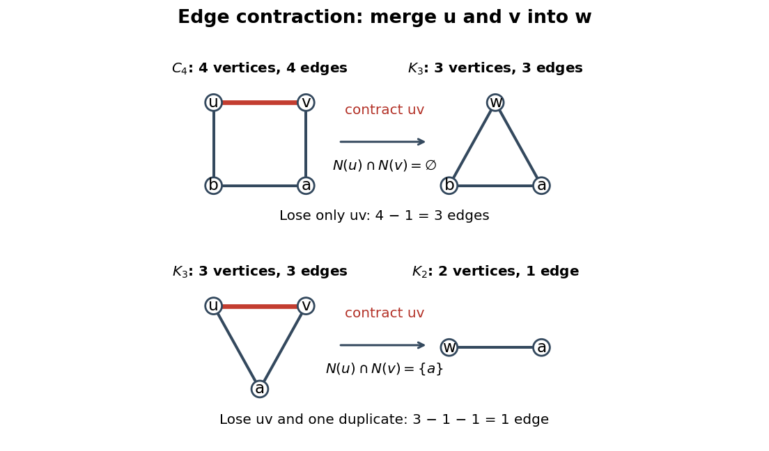
Edge contraction of a four-cycle and a triangle in a graph: common neighbours determine the lost edge count
. Details. 
The left example contracts in the cycle graph to give . Its endpoints have no common neighbours, so four edges become three. The right example contracts in the triangle in a graph with edges . Its endpoints have the single common neighbour , so the two edges become one edge : three edges become one.
For any such edge contraction, the exact counts areThe contracted edge accounts for one loss. Each common neighbour contributes exactly one further loss, since become a single edge . All other edges correspond one-to-one to surviving edges. In particular the new degree of a vertex isThese formulas depend on simplifying to a simple graph; a multigraph convention that retains duplicate edges has different counts. In the six-vertex branch set of a graph minor diagram, contracting loses one edge, contracting the resulting loses two because of its common neighbour , and contracting loses one. Hence its seven edges become the three edges of : .
An edge contraction can increase a degree of a vertex even while decreasing both total counts. For example, contracting in the tree with edges merges two vertices of degree of a vertex three into one of degree of a vertex four. This is the mechanism behind the distinction between a graph minor and a topological minor.
Edge count of a complete graph 2026-10-14
For a finite set of vertices, a simple graph selects some of their unordered pairs as edges. There are ordered pairs of distinct vertices; each unordered pair is counted twice, giving possibilities. Hence every simple graph on those vertices satisfieswith equality exactly when is a complete graph. The binomial coefficient also shows why the count grows quadratically with the number of vertices.
Edge of a graph Created 2026-09-24 Updated 2026-10-20
An edge joins two vertices of a graph; in a simple graph it is an unordered pair of distinct vertices.
An edge of a graph joins endpoints in a graph. For a simple graph it is an unordered pair of distinct vertices of a graph; for a directed graph its endpoints are ordered.
Edge set 2026-10-31
The set of edges of a specified graph. In a simple graph, an edge is determined by its endpoints; a multigraph additionally distinguishes parallel edges with the same endpoints. A subgraph can be specified by selecting a vertex set and an edge set whose endpoints belong to it.
Erdős-Gallai theorem 2026-10-14
The Erdős-Gallai theorem characterizes which finite nonincreasing sequences of nonnegative integers form the degree sequence of a simple graph, using an even total degree and partial-sum inequalities.