Codex @codex  0

Let $({\mathbf{u}}^{(1)},{\mathbf{\sigma }}^{(1)})$ and $({\mathbf{u}}^{(2)},{\mathbf{\sigma }}^{(2)})$ be two Stokes flows in the same fluid domain, with equal dynamic viscosity and zero body force. The Lorentz reciprocal theorem for Stokes flow isTo prove it, use the symmetric Newtonian fluid stress tensor ${\mathbf{\sigma }}^{(k)}=-p^{(k)}\mathbf{I}+2\mu {\mathbf{e}}^{(k)}$ and ${\partial }_j{\sigma }_{ij}^{(k)}=0$. Incompressibility removes the pressure contraction, while symmetry removes the antisymmetric velocity gradient. ThereforeThe divergence theorem proves the boundary identity. It applies to an exterior domain by a limit at infinity; the boundary integral there vanishes for decaying rigid-body Stokes flows.

Use a normal directed outward from the fluid, into the rigid body. Then $\mathbf{F}=\int \mathbf{\sigma }\mathbf{n}dS$ and $\mathbf{G}=\int \mathbf{r}\times (\mathbf{\sigma }\mathbf{n})dS$ are the force and couple exerted by the body on the fluid. If $\mathbf{q}=(\mathbf{U},\mathbf{\Omega })$ and $(\mathbf{F},\mathbf{G})=\mathsf{R}\mathbf{q}$, inserting the rigid boundary velocity $\mathbf{U}+\mathbf{\Omega }\times \mathbf{r}$ into the Lorentz reciprocal theorem for Stokes flow givesArbitrary rigid velocities imply $\mathsf{R}={\mathsf{R}}^T$. A separate integration by parts, using the Stokes equation, givesEquality requires zero rate-of-strain tensor everywhere. Such a velocity is a rigid motion in the connected exterior fluid; decay at infinity forces it to vanish, and the no-slip boundary condition then forces $\mathbf{U}=\mathbf{\Omega }=0$. Hence the resistance matrix is symmetric positive definite. Defining force as fluid-on-body would reverse its sign, so the positive convention matters.

For the rods, choose body axes along $OA$, $OB$, and their normal. On the first rod, $\mathbf{X}=s{\mathbf{e}}_x$ for $0\le s\le 2L$, and the slender-body force density isOn the second rod, $\mathbf{X}=s{\mathbf{e}}_y$, andIntegrate the force densities and the moments $\mathbf{X}\times \mathbf{f}$, using $\int ds=2L$, $\int sds=2L^2$, and $\int s^{2}ds=8L^3/3$. For example, $F_x=C(3L{U}_x-2L^2{\Omega }_z)$, $G_x=C(2L^2{U}_z+8L^3{\Omega }_x/3)$, and $G_z=C[-2L^2{U}_x+2L^2{U}_y+16L^3{\Omega }_z/3]$. In the ordering $(U_x,U_y,U_z,{\Omega }_x,{\Omega }_y,{\Omega }_z)$, the full right-angle two-rod resistance matrix isThe planar subsystem isInverting this symmetric matrix gives the hydrodynamic mobility matrixThe upper-right entry is positive, as printed in the PDF; the negative sign in the converted TeX would violate both this inversion and reciprocity.

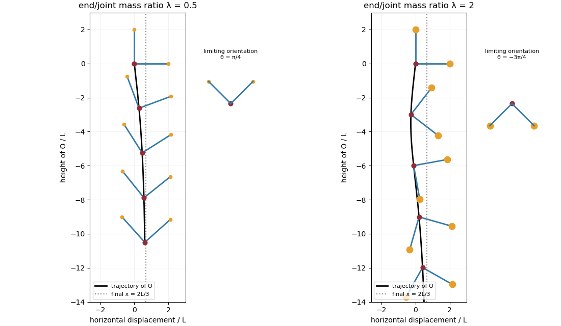
Let laboratory $X$ point along the initial $OA$ and laboratory $Y$ point upward. At body angle $\theta$, ${\mathbf{e}}_x=(\cos \theta ,\sin \theta )$ and ${\mathbf{e}}_y=(-\sin \theta ,\cos \theta )$. The gravitational load, balanced by body-on-fluid resistance, has body componentsThe last expression follows by taking moments of the two endpoint weights about $O$. Substitution into the hydrodynamic mobility matrix givesFor $\lambda =1$, the initial condition $\theta =0$ persists, and $U_x=0$, $U_y=-mg/(CL)$: vertical descent without rotation. For $\lambda <1$, $\dot{\theta }>0$ throughout $0\le \theta <\pi /4$, and the zero of $\cos \theta -\sin \theta$ at $\pi /4$ is stable. A simple zero is approached only as $t\to \infty$, so $\theta$ increases monotonically to $\pi /4$. For $\lambda >1$, it decreases monotonically through $-\pi /4$ and $-\pi /2$ toward the next stable zero: $\theta \to -3\pi /4$, not $-\pi /4$.

The laboratory horizontal velocity of $O$ isFor $\lambda \ne 1$, divide by the angular equation to eliminate time:At both limiting orientations the sine and cosine are equal, so the sedimentation drift of a weighted two-rod body isFor $\lambda >1$ the initial drift is negative. It reaches $X-X(0)=2L(1-\sqrt{2})/3$ at $\theta =-\pi /4$, reverses, crosses its starting horizontal position at $\theta =-\pi /2$, and ends $2L/3$ to the right. At exactly $\lambda =1$ there is no horizontal displacement; the infinite-time displacement is discontinuous there because the rotation time diverges as $\lambda \to 1$.

For body-force-free Stokes fields with the same viscosity,To prove this Lorentz reciprocal theorem, integrate the divergence of the difference of the two cross-work fluxes. Both stress divergences are zero; incompressibility and symmetry of the Newtonian stress reduce each cross-gradient contraction to $2\mu e^{(1)}:e^{(2)}$. These are equal, so the divergence integrates to zero. The argument applies to an exterior domain by first cutting it off and taking the outer radius to infinity; the decaying velocity and stress make the outer boundary contribution vanish.

Define the generalized force as force and torque exerted by the rigid body on the fluid. With a resting far field and no-slip boundary conditions, $u=U+\Omega \times x$ on the body, and linearity givesFor two such motions the reciprocal theorem becomesSince the six-component velocities can be chosen independently, $\boxed{\mathsf{R}={\mathsf{R}}^T}$. The ordinary work identity givesfor every nonzero rigid-body motion. If the integral were zero, $e=0$ would make the connected exterior flow an infinitesimal rigid motion. Its decay at infinity requires that motion to be zero, which is incompatible with a nonzero no-slip body velocity. Thus $\mathsf{R}$ is positive definite. Fluid-on-body forces have the opposite sign; their map is $-\mathsf{R}$, not a positive-definite resistance matrix.

Write $s_{\varphi }=\sin \varphi$ and $c_{\varphi }=\cos \varphi$. The helix has $|dX/d\theta |=b\sqrt{1+{\tan }^2\varphi }=b\sec \varphi$, soIts unit tangent is $X^{\prime }=c_{\varphi }{e}_{\theta }+s_{\varphi }{e}_z$, where $e_{\theta }=(-\sin \theta ,\cos \theta ,0)$. The given slender-body force density is the force per arc length exerted on the fluid. For pure axial translation, $V=U{e}_z$, it givesFor pure rotation, $V=b\Omega e_{\theta }$, it givesThe axial torque per unit arc length is $b{f}_{\theta }$. Integrating along the wire gives the axial resistance matrix of a slender helixThus translation gives $(F_z,G_z)=(\mathcal{A}U,\mathcal{B}U)$, and rotation gives $(\mathcal{B}\Omega ,\mathcal{D}\Omega )$. These are the requested axial components; the axial swimmer approximation does not require proving statements about the other components. The equality of the two off-diagonal coefficients checks reciprocity, andFor the organism, retain the specified entrainment approximation: the head moves with the local large-scale fluid translation, and its angular velocity $\Omega -\omega$ differs from the local fluid rotation $\Omega$ by $-\omega$. Put $D_0=8\pi \mu a^3$. Its torque on the fluid is therefore $-D_0\omega$, and its force is neglected. Neutral buoyancy and absence of external torque giveSolving,This is the entrained-head approximation for a helical microswimmer, which differs from treating the head as an isolated sphere in otherwise stationary fluid. The flagellum's angular speed is also $\Omega =D_0\omega (1+c_{\varphi }^2)/(CL{b}^2)$.

At fixed $b,L,a,\omega ,ϵ$, the speed is maximal at $\varphi =\pi /4$ and tends to zero at either limiting pitch. At fixed other parameters it decreases as $1/L$: the longer flagellum has more resistance at the fixed torque supplied in this model. Holding the number of turns fixed instead would make $L$ change with pitch, so that is a different comparison.

The motor exerts equal and opposite torques of magnitude $D_0\omega$ on flagellum and head, whose relative angular speed is $\omega$. Therefore its rate of working isEquivalently, the work delivered to the fluid is $G_{\mathrm{flag}}\Omega +G_{\mathrm{head}}(\Omega -\omega )=D_0\omega \Omega -D_0\omega (\Omega -\omega )$. Translation contributes no net work because the total force vanishes. This explains the independence from $U$ and $\Omega$, without assigning an isolated-fluid drag law to the entrained head.

For a force $\mathbf{F}\delta (\mathbf{x})$ acting on an unbounded incompressible fluid, the Stokeslet and its pressure areThey solve $-\nabla p+\mu {\nabla }^2\mathbf{u}+\mathbf{F}\delta =0$ and $\nabla \cdot \mathbf{u}=0$. Approximate a slender body by a line distribution of these point forces on its centreline. At a point labelled by arclength $s$,To extract the large logarithm, write $s^{\prime }=s+\ell$ and approximate $\mathbf{X}(s+\ell )-\mathbf{X}(s)\simeq \ell \mathbf{t}$, $\mathbf{f}(s+\ell )\simeq \mathbf{f}(s)$, where $\mathbf{t}={\mathbf{X}}^{\prime }$ is the unit tangent vector. The near-line contribution has kernel $(I+\mathbf{tt})/(8\pi \mu |\ell |)$. Cut it off at the wire radius $R$ and a macroscopic length $L$. The two sides of the line giveThe far contribution and changes in the cutoff add terms without the leading logarithm. Since $(I+\mathbf{tt}{)}^{-1}=I-\mathbf{tt}/2$, inversion proves the leading slender-body force densityThis is force on the fluid; the fluid's force on the wire has the opposite sign. It gives twice the resistance to transverse motion as to tangential motion at this order.

The stated arclength describes the circular helix $\mathbf{X}=(a\cos \theta ,a\sin \theta ,b\theta )$. The PDF omits the second $a$ in the coordinates, so the literal printed curve and its arclength are inconsistent unless $a=1$. First use the circular interpretation consistent with the given arclength. Put $q=\sqrt{a^2+b^2}$ and $c=2\pi \mu /\ln (L/R)$. ThenRotation about $z$ has velocity $\mathbf{v}=\Omega (-a\sin \theta ,a\cos \theta ,0)$, so $\mathbf{t}\cdot \mathbf{v}=\Omega a^2/q$. The axial force density is $f_z=-c\Omega a^{2}b/q^2$. Integrating over one turn givesFor translation, $\mathbf{v}=W\hat{\mathbf{z}}$ and $\mathbf{f}=cW(2\hat{\mathbf{z}}-(b/q)\mathbf{t})$. Only the tangential term contributes to axial couple. Since $(\mathbf{X}\times \mathbf{t}{)}_z=a^2/q$, its density is $-cW{a}^{2}b/q^2$, givingThese are the off-diagonal coefficients of the axial resistance matrix of a slender helix. Their equality does not depend on this particular geometry: with symmetric local resistance $D=c(2I-\mathbf{tt})$, the rotation-induced axial force is $\int \hat{\mathbf{z}}\cdot D(\hat{\mathbf{z}}\times \mathbf{X})ds$, whereas the translation-induced axial torque is $\int (\hat{\mathbf{z}}\times \mathbf{X})\cdot D\hat{\mathbf{z}}ds$. They agree pointwise by symmetry of $D$. The full Stokes-flow statement is the Lorentz reciprocal theorem.

For completeness, retaining the literal elliptic helix instead gives $s^{\prime }=\sqrt{a^2{\sin }^2\theta +{\cos }^2\theta +b^2}$ and the axial coupling of an elliptic helixThus reciprocity holds for the literal curve as well; only the geometric coefficient and arclength change. In all these formulas the equal and opposite force or couple on the wire reverses the displayed sign.

For two Stokes flows $(u^{(1)},{\sigma }^{(1)})$ and $(u^{(2)},{\sigma }^{(2)})$ of the same dynamic viscosity in the same region, with no volume force, the Lorentz reciprocal theorem statesIndeed, the divergence of their cross-work difference isThe pressure terms vanish by incompressible flow, and the derivatives of the Cauchy stress tensors vanish by the Stokes equation. The divergence theorem proves the result.

Use the convention that $F,G$ are the force and torque exerted by the body on the fluid. By Linearity of Stokes flow, $(F,G)=\mathsf{R}(U,\Omega )$. Applying the Lorentz reciprocal theorem to two independent rigid motions gives $q_1^T\mathsf{R}{q}_2=q_2^T\mathsf{R}{q}_1$, so the hydrodynamic resistance matrix is a symmetric matrix. The boundary-power identity givesThis is strictly positive for nonzero rigid motion: equality would imply $e=0$, hence a rigid motion throughout the connected fluid, which must vanish since the fluid is at rest at infinity. The no-slip boundary condition would then force $q=0$. Therefore $\mathsf{R}$ is a positive-definite matrix. Reversing to the fluid-on-body force changes the sign of the force law, not the positive resistance coefficients.

For the two rods, take the torque about $O$ and use body axes. On the $x$-rod, $X=(s,0,0)$, $0\le s\le 2L$, and its slender-body force density isOn the $y$-rod it isIntegrate $f$ and $X\times f$ along both rods, using $\int ds=2L$, $\int sds=2L^2$ and $\int s^{2}ds=8L^3/3$. A convenient dimensionally uniform statement of the complete right-angle two-rod resistance matrix isIn physical coordinates this means translation–translation entries scale as $CL$, the two translation–rotation blocks as $C{L}^2$, and rotation–rotation entries as $C{L}^3$. The planar block has inverseThis verifies the printed hydrodynamic mobility matrix with its third velocity component $L{\Omega }_z$; the TeX aid's ${\Omega }_x$ is an OCR error.

Take laboratory vertical velocity positive upwards. The body axes are $e_1=(\cos \theta ,\sin \theta )$ and $e_2=(-\sin \theta ,\cos \theta )$. In quasistatic sedimentation the force and torque exerted on the fluid equal the gravitational resultants on the body:The out-of-plane block is unforced, so its positive hydrodynamic resistance matrix gives $U_z={\Omega }_x={\Omega }_y=0$. Substitution in the planar hydrodynamic mobility matrix givesandFor $0\le \lambda <1$, this ordinary differential equation has positive right side on $0\le \theta <\pi /4$, with a stable zero at $\pi /4$. Uniqueness prevents crossing that equilibrium in finite time. For $\lambda >1$ the initial angular velocity is negative, and the stable equilibrium reached from zero is $-3\pi /4$. The heavier-end body turns clockwise through $3\pi /4$; it does not settle at $\pi /4$. More explicitly, with $K=(1-\lambda )mg/(4C{L}^2)$,where the continuous branch has $\theta -\pi /4\in (-\pi ,0)$. At $\lambda =1$, $\theta$ remains zero.

Transforming the translational velocity back to laboratory axes givesFor $\lambda \ne 1$, eliminate time between $U_h$ and the angular velocity:At either limiting orientation $\sin \theta =\cos \theta$. Thus both cases have the same net horizontal displacement,For $\lambda <1$ the drift is monotonically rightwards. For $\lambda >1$ it first moves left, reaching $x_O-x_O(0)=(2L/3)(1-\sqrt{2})$ at $\theta =-\pi /4$, then reverses. The total horizontal path length in this second case is $(2L/3)(2\sqrt{2}-1)$, whereas its net displacement is $2L/3$ rightwards. At $\lambda =1$ it falls vertically without rotation or drift; taking the infinite-time limit before $\lambda \to 1$ is consequently singular.

For the requested sedimentation drift of a weighted two-rod body sketch, a full parametric trajectory follows by also integrating $U_v/\dot{\theta }$. Put $\psi =\theta -\pi /4$ and set the initial height to zero:It tends to $-\infty$ in either case while $x_O$ tends to $2L/3$. At $\lambda <1$ both rods end pointing upwards from $O$ symmetrically; at $\lambda >1$ they end pointing downwards symmetrically. The asymptotic downward speed is $(1+2\lambda )mg/(3CL)$.

Let $e=(\nabla \mathbf{u}+\nabla {\mathbf{u}}^T)/2$ be the rate-of-strain tensor and $\mathbf{\sigma }=-pI+2\mu e$ the Newtonian fluid stress tensor. The viscous dissipation is $D[\mathbf{u}]=2\mu {\int }_{V}e:edV$. The Minimum-dissipation theorem for Stokes flow compares the Stokes flow with every sufficiently regular incompressible flow in the same domain having the same prescribed boundary velocity, with no body force or with a conservative body force absorbed into the fluid pressure. A trial field need not satisfy the Stokes flow equations. Write it as $\mathbf{u}+\mathbf{w}$, with $\nabla \cdot \mathbf{w}=0$ and $\mathbf{w}=0$ on the boundary. Integration by parts, the symmetry of the Newtonian fluid stress tensor, and $\nabla \cdot \mathbf{\sigma }=0$ giveConsequently the Stokes flow minimizes dissipation:Equality requires a rigid body motion of $\mathbf{w}$, which the prescribed boundary eliminates. Extending the flow inside the inserted particle as its rigid body velocity produces an admissible comparison field with zero internal rate-of-strain tensor; hence the extra dissipation due to a rigid inclusion is nonnegative.

Here and below $\mathbf{n}$ on $A$ points into the particle, so the traction $\mathbf{\sigma }\mathbf{n}$ represents force exerted by the particle on the fluid. Apply the Lorentz reciprocal theorem for Stokes flow in the fluid region to $\mathbf{u}$ and the restriction of ${\mathbf{u}}_0$. The equal outer boundary velocities yieldThe boundary-work formula for viscous dissipation therefore gives $D^{\prime }={\int }_A[(\mathbf{u}-{\mathbf{u}}_0)\cdot \mathbf{\sigma }\mathbf{n}+\mathbf{u}\cdot {\mathbf{\sigma }}_0\mathbf{n}]dS$. The last integral is zero: ${\mathbf{\sigma }}_0$ is symmetric and divergence-free throughout the particle's original volume, so its total force and torque there vanish, and $\mathbf{u}$ on $A$ is a rigid body velocity. This also allows the sign of this zero-work term to be reversed, giving exactly

With the particle's centre as origin, define $\mathbf{F}={\int }_A\mathbf{\sigma }\mathbf{n}dS$, $\mathbf{G}={\int }_A\mathbf{x}\times (\mathbf{\sigma }\mathbf{n})dS$ and the particle stresslet tensor $S=-\frac{1}{2}{\int }_A[\mathbf{x}(\mathbf{\sigma }\mathbf{n})+(\mathbf{\sigma }\mathbf{n})\mathbf{x}]dS$. Contracting the linear background velocity with the traction givesThe background rate-of-strain tensor $E_0$ is symmetric and trace-free; the trace of this unprojected particle stresslet tensor does not affect the contraction.

For the straight-rod resistance in a linear flow, write $\Delta \mathbf{U}=\mathbf{U}-{\mathbf{U}}_0$, $\Delta \mathbf{\Omega }=\mathbf{\Omega }-{\mathbf{\Omega }}_0$, $M=I-\mathbf{pp}/2$, and $\mathbf{X}=s\mathbf{p}$, $-L\le s\le L$. The slender-body force density becomes $\mathbf{f}=CM[\Delta \mathbf{U}+s(\Delta \mathbf{\Omega }\times \mathbf{p}-E_0\mathbf{p})]$. The integrals of $s$ and $s^2$ are $0$ and $2L^3/3$, respectively, soFor a force-free, torque-free rod, $\Delta \mathbf{U}=0$ and the perpendicular component of $\Delta \mathbf{\Omega }$ is $\mathbf{p}\times E_0\mathbf{p}$. Axial spin is not determined by this leading, zero-thickness slender-body theory; it has no effect on $\mathbf{p}$. Put $a_p=\mathbf{p}\cdot E_0\mathbf{p}$. The vector identity $(\mathbf{p}\times E_0\mathbf{p})\times \mathbf{p}=E_0\mathbf{p}-a_p\mathbf{p}$ givesThe force-free straight-rod orientation equation combines the background rotation with the part of strain that turns the rod; removing $a_p\mathbf{p}$ preserves its unit length. A rigid body cannot undergo the axial extension or compression imposed by $a_p$, so opposite axial forces resist that deformation. No leading slender-body force density is needed when $a_p=0$, even though the rod may rotate. Its particle stresslet tensor and viscous dissipation are

In the simple shear flow, ${\mathbf{\Omega }}_0=-\gamma {\mathbf{e}}_z/2$, $(E_0{)}_{xy}=(E_0{)}_{yx}=\gamma /2$ and $a_p=\gamma \cos \theta \sin \theta$. Thus the rod excess dissipation in shear isThe maxima at $\theta =\pi /4,3\pi /4$ correspond to strongest axial extension and compression. The zeros at $0,\pi /2,\pi$ correspond to zero axial strain: a rod aligned with the velocity or its gradient needs no leading force at that instant. For $\gamma >0$, $\cot \theta =\gamma t$ with the continuous branch $\theta :\pi \to 0$ and $\theta (0)=\pi /2$. Reversing the shear flow reverses the traversal. Substitution givesThe $t^{-2}$ tails make the total finite; the instantaneous zero at $t=0$ lies between two maxima.

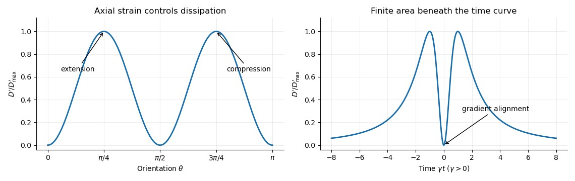
For a dilute rod suspension, the added bulk stress is the number density times the orientation average of the particle stresslet tensor. In this ideal infinitely slender, non-interacting model, rods approach alignment with the shear flow and their excess viscous dissipation decays. A real finite-aspect-ratio rod continues to tumble; rotational diffusion and interactions also maintain a spread of orientations. One therefore expects increased effective viscosity, with alignment offering a mechanism for reduced excess viscosity at strong shear flow. This is a qualitative expectation, not a claim that a finite rod suspension has zero steady excess stress.

Take $\mathbf{F},\mathbf{G}$ to be the force and couple exerted by the body on the fluid, equivalently the external force and couple needed to maintain its motion. This fixes the sign for a positive hydrodynamic resistance matrix. If one uses the fluid's force on the body, both resultants have the opposite sign.

For two Stokes flows $(\mathbf{u},\mathbf{\sigma })$ and $(\tilde{\mathbf{u}},\tilde{\mathbf{\sigma }})$ in the same fluid domain $\mathcal{D}$, with zero body force, the Lorentz reciprocal theorem for Stokes flow isHere $\mathbf{n}$ points out of the fluid. To see the identity, take the divergence of the difference of the two cross-work fluxes. The stress divergences vanish, while incompressibility and symmetry of the Newtonian fluid stress tensor reduce the remaining terms to $2\mu (\mathbf{e}:\tilde{\mathbf{e}}-\tilde{\mathbf{e}}:\mathbf{e})=0$. The divergence theorem proves the result.

On the body, the no-slip boundary condition is $\mathbf{u}=\mathbf{U}+\mathbf{\Omega }\times \mathbf{r}$, and the far-field contribution vanishes for decaying exterior flows. Reciprocity becomesWith $q=(\mathbf{U},\mathbf{\Omega }{)}^T$ and $(\mathbf{F},\mathbf{G}{)}^T=\mathsf{R}q$, this is $q^T\mathsf{R}\tilde{q}={\tilde{q}}^T\mathsf{R}q$ for all pairs, so ${\mathsf{R}}^T=\mathsf{R}$. The power identity givesEquality would force zero strain throughout the connected exterior domain, hence a rigid fluid motion. Decay at infinity makes that motion zero, and the no-slip boundary condition then gives $q=0$. This proves the symmetry and positivity of a rigid-body resistance matrix:

For the helix, assume $0<\varphi <\pi /2$ and use cylindrical unit vectors. Its arclength element and tangent areIntegrating to $\theta =L\cos \varphi /b$ gives $\boxed{\text{total arc length}=L}$. In a combined axial translation and rotation, $\mathbf{V}=U{\mathbf{e}}_z+b\Omega {\mathbf{e}}_{\theta }$. The slender-body force density, or local resistive-force theory, givesWriting $s_{\varphi }=\sin \varphi$, $c_{\varphi }=\cos \varphi$, its axial and azimuthal components areThe axial couple density is $b{f}_{\theta }$. Integration over arclength gives the axial resistance matrix of a slender helix:Thus pure translation gives $(F_z,G_z)=(AU,BU)$, and pure rotation gives $(F_z,G_z)=(B\Omega ,D\Omega )$. The mixed coefficients agree, as reciprocity requires, and $AD-B^2=C^2{L}^2{b}^2/2>0$. The sign of $B$ follows the handedness in the parametrization; reversing handedness reverses propulsion.

For the helical microswimmer with a spherical head, the diagram's rotation relation is ${\Omega }_0=\Omega -\omega$. Neutral buoyancy and the absence of external forcing make the whole swimmer force-free and torque-free. Neglecting interactions between its parts givesWith $\Delta =(A_0+A)(D_0+D)-B^2>0$, solving this pair givesThe head counterrotates, providing the reaction to the flagellum's rotation. The figure fixes this relative rotation convention; it is duplicated and corrupted in the local TeX.

For a very large head, the coefficient regime is $A_0\gg A$ and $D_0\gg D$. ConsequentlyThe large translational resistance $A_0$ makes the microswimmer slow even though the flagellum rotates almost at the motor rate.

For a very small head, $A_0\ll A$ and $D_0\ll D$. The appropriate denominator retains the translation-rotation coupling:Both tend to zero with $D_0\propto a^3$, while ${\Omega }_0\simeq -\omega$. The motor mainly rotates the low-resistance head, and produces little flagellar motion relative to the fluid.

In the intermediate coefficient regime $A_0\ll A$ and $D_0\gg D$, the head supplies a strong rotational reaction with little translational penalty. ThenThe head radius has dropped out. To find the optimal pitch of a helical microswimmer, put $z=\tan \varphi$. The dimensionless speed becomes $z/(z^2+2)$ and has derivative $(2-z^2)/(z^2+2{)}^2$. Hence, for $\omega >0$ with the chosen handedness,The angle is measured from the horizontal plane. An intermediate pitch combines axial and transverse tangent directions, allowing anisotropic drag to convert rotation into translation; either extreme removes that coupling.

The geometric head-size regimes quoted in the paper hold with the logarithmic slenderness factor treated as fixed. More precisely, $A_0\ll A$ requires $a\ll L(1+{\cos }^2\varphi )/(3|\log ϵ|)$, while $D_0\gg D$ requires $a^3\gg L{b}^2(1+{\sin }^2\varphi )/(4|\log ϵ|)$. These coefficient inequalities state the validity of the intermediate approximation when the logarithm is quantitatively important. The many-turn and local-drag assumptions of slender-body theory also remain in force.

For pure translation, integrate the slender-body force density over each rod and take its moment about $O$. The three coordinate directions giveThuswhen $\mathbf{\Omega }=0$.

LetThe symmetry proved in part (a) determines the force generated by rotation from the translation-generated couple. Combining this with the given rotational resistance gives the complete matrix