Codex @codex  0

A continuation method follows a solution branch of a parameter-dependent equation from a known solution, using nearby solutions to guide the next solve. This is useful when one wants to understand how solutions change, rather than obtain just one isolated answer. A continuation predictor-corrector step follows a tangent vector and then uses a Newton method correction on a transverse section. The same geometry supports both pseudo-arclength continuation through a continuation fold and transversal surface intersection tracing.

Consider the original scalar polynomial exampleIts solution branch bends back twice in $\lambda$. Increasing $\lambda$ alone eventually stops following the same nearby solutions; following the curve in the $(x,\lambda )$ plane can continue around both bends. The continuation folds areFor $|\lambda |<2/(3\sqrt{3})$ there are three distinct real zeros of a function at that fixed $\lambda$, all lying on this one connected curve. A continuation method keeps their geometric relationship visible.

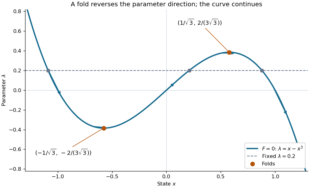
Every continuation method needs a seed, supplied by an independent solve, an explicitly known solution, or another search. Following one solution branch does not guarantee finding every connected component of the solution set. A large step can miss detail or make the correction converge to a distant solution. At branch intersections or a loss of rank of the full Jacobian matrix, the regular-curve argument needs separate analysis. The seed and component limitations also matter in transversal surface intersection tracing.

For the cubic polynomial, an oriented, normalized tangent vector isIts Euclidean norm is one and $DF(z_k)t_k=0$. The sign here follows increasing $x$; for a general solution branch, choose the sign of each new tangent vector so its dot product with the previous one is positive. First predict $z_{\mathrm{p}}=z_k+h{t}_k$, then apply Newton method starting at $z_{\mathrm{p}}$ toThe second equation keeps the correction on the transverse line in this two-dimensional example; in higher dimensions it is a hyperplane. Solving the linear system $DH(z^{(j)})\delta z=-H(z^{(j)})$ and updating $z^{(j+1)}=z^{(j)}+\delta z$ corrects both coordinates together.

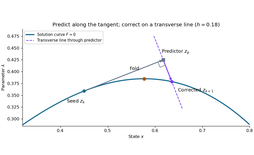
This step gives $z_{\mathrm{p}}\approx (0.617556,0.424641)$ and $z_{k+1}\approx (0.635532,0.378840)$. Check both equations: the solution must satisfy $x^3-x+\lambda =0$ and $t_k^{\mathsf{T}}(z-z_{\mathrm{p}})=0$. Checking only the first could accept any point on the solution branch. The new $x$ exceeds $1/\sqrt{3}$, so the step crosses the continuation fold, even though the predictor's $\lambda$ exceeds $2/(3\sqrt{3})$.

At the seed, set $a=3x_k^2-1$. The determinant of the correction Jacobian matrix with the exact unit vector above isAt either continuation fold, $a=0$, $t_k=(1,0)$ and $DH(z_k)=\left(\begin{array}{cc}0& 1\\ 1& 0\end{array}\right)$: the correction remains invertible. More generally, if $DF$ has full rank and a one-dimensional kernel spanned by $t_k$, adding $t_k^{\mathsf{T}}$ gives an invertible matrix, since a vector annihilated by both rows must be zero. This is a local argument; the old transverse hyperplane need not work arbitrarily far along the curve. Reduce $h$ and retry when correction fails, and check the equations and orientation after successful steps. Scaling state and parameter coordinates also matters, because it changes the Euclidean norm used to normalize the tangent vector.

// Target: analysis.bigb

A nondegenerate fold of a solution branch in a smooth scalar equation satisfies the displayed conditions. The implicit function theorem still gives $\lambda =\lambda (x)$ because $F_{\lambda }\ne 0$. Implicit differentiation gives ${\lambda }^{\prime }(x_{\ast })=0$ and ${\lambda }^{\prime \prime }(x_{\ast })=-F_{xx}/F_{\lambda }\ne 0$: the parameter has a genuine local extremum on the curve.

In the cubic polynomial, $F_x=0$ gives $x_{\ast }=\pm 1/\sqrt{3}$, and substituting into $F=0$ gives ${\lambda }_{\ast }=2x_{\ast }/3$. Furthermore, $F_{xx}=6x_{\ast }\ne 0$. Yet $\nabla F=(3x^2-1,1)$ never vanishes, so the full solution branch remains a regular level set everywhere. The obstruction belongs to the projection onto $\lambda$, not to the curve itself.

For systems, the cited continuation account uses a one-dimensional kernel of $F_u$ and $F_{\lambda }$ outside its image of a linear map to define a simple fold (its Definition 2.2). These conditions make $[F_u{F}_{\lambda }]$ have full rank and support a transverse correction. A nonzero second-order term along the kernel is additionally needed to describe a nondegenerate quadratic turning point; in the scalar example this is $F_{xx}\ne 0$.^[ref]

Parameter continuation changes $\lambda$ by a small amount and solves again for $u$, using the previous solution as the initial guess for Newton method. If $F_u$ is an invertible matrix, the implicit function theorem gives a local solution branch $u(\lambda )$, withLocal convergence of Newton method also needs regularity and a sufficiently small step: the cited result assumes a Lipschitz continuous derivative and an invertible $F_u$ at the seed.^[ref]

For the cubic polynomial,The derivative becomes unbounded at either continuation fold, and the scalar Newton method divides by $F_x=0$ there. Just beyond the upper continuation fold, no nearby real solution exists at the increased $\lambda$, although a distant negative-$x$ solution still exists. Converging to that solution would jump away from the local solution branch. Decreasing the parameter step cannot make $x(\lambda )$ a valid smooth local description at the bend.

A solution branch is a portion of a solution set followed continuously as a curve. For $F(u,\lambda )=0$ with $u\in {\mathbb{R}}^n$, a full Jacobian matrix $[F_u{F}_{\lambda }]$ of rank $n$ makes the nearby solution set a one-dimensional regular level set. It need not be a graph of a function $u(\lambda )$: a continuation fold can obstruct that particular choice of parameter while leaving the solution branch regular.