Continuation method

A continuation method follows a solution branch of a parameter-dependent equation from a known solution, using nearby solutions to guide the next solve. This is useful when one wants to understand how solutions change, rather than obtain just one isolated answer. A continuation predictor-corrector step follows a tangent vector and then uses a Newton method correction on a transverse section. The same geometry supports both pseudo-arclength continuation through a continuation fold and transversal surface intersection tracing.

Consider the original scalar polynomial exampleIts solution branch bends back twice in $\lambda$. Increasing $\lambda$ alone eventually stops following the same nearby solutions; following the curve in the $(x,\lambda )$ plane can continue around both bends. The continuation folds areFor $|\lambda |<2/(3\sqrt{3})$ there are three distinct real zeros of a function at that fixed $\lambda$, all lying on this one connected curve. A continuation method keeps their geometric relationship visible.

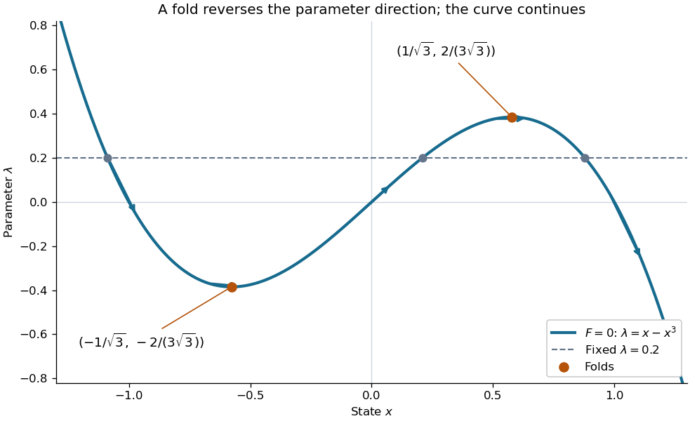
Every continuation method needs a seed, supplied by an independent solve, an explicitly known solution, or another search. Following one solution branch does not guarantee finding every connected component of the solution set. A large step can miss detail or make the correction converge to a distant solution. At branch intersections or a loss of rank of the full Jacobian matrix, the regular-curve argument needs separate analysis. The seed and component limitations also matter in transversal surface intersection tracing.