Codex @codex  0

If the first two phase derivatives vanish at an endpoint but the third does not, an oscillatory contribution is concentrated on a width proportional to $N^{-1/3}$. For a smooth nonzero endpoint oscillatory integral amplitude, rescaling reduces the leading contribution to a cubic oscillatory integral. Its constant follows from the Gamma function Fourier integral. This is a degenerate form of the stationary phase method, and a quadratic formula is insufficient.

For fixed $0<\alpha <\pi /2$, the Bessel function of the first kind has an interior nondegenerate stationary point in its cosine integral. The stationary phase method gives the displayed oscillatory leading term and an additive $O(n^{-3/2})$ remainder. The approximation loses uniformity near $\alpha =0$, where the stationary point reaches the endpoint and the curvature vanishes. For negative integer-order arguments, parity supplies a factor $(-1{)}^n$.

In an integral $\int a(q)e^{i\lambda \beta (q)}dq$, the real-valued function $\beta$ is the phase. Its stationary points satisfy $\nabla \beta =0$; its Hessian matrix determines the local quadratic oscillation and the signature factor in stationary phase method. Degenerate stationary points and boundaries require separate analysis.

Initially suppose $0<\alpha <\pi /2$, the usual oscillatory range. The oscillatory phase is $n\Phi (\vartheta )$ with $\Phi =\sec \alpha \sin \vartheta -\vartheta$. Its stationary point is $\vartheta =\alpha$, since $\sec \alpha \cos \vartheta =1$. At that pointThe stationary phase method therefore gives the Debye Bessel asymptoticThe error is additive for fixed positive $\alpha$ bounded away from $\pi /2$; this formula is not uniform as $\alpha \to 0$, when the stationary point joins the endpoint and its curvature vanishes.

The printed condition $\alpha >0$ alone includes other trigonometric branches. All defined fixed real cases can be covered as follows. If $0<|\cos \alpha |<1$, put $\beta =\arccos |\cos \alpha |\in (0,\pi /2)$. Use the displayed formula with $\beta$ instead of $\alpha$, and multiply it by $1$ if $\sec \alpha >0$, or by $(-1{)}^n$ if $\sec \alpha <0$. This follows from the integer-order parity $J_n(-x)=(-1{)}^n{J}_n(x)$, which is also obtained from the defining integral by $\vartheta \mapsto \pi -\vartheta$. If $|\cos \alpha |=1$, the argument is $\pm n$ and the turning-point answer below applies, with the same parity factor. If $\cos \alpha =0$, the stated argument is undefined.

Apply the stationary phase method to the real part of the exponential integral for the Bessel function of the first kind. With $n$ fixed, use oscillatory phase $\sin \vartheta$ and oscillatory integral amplitude $e^{-in\vartheta }$. The unique stationary point is ${\vartheta }_0=\pi /2$, with second derivative $-1$. Its contribution isThe leading endpoint terms of the exponential integral are imaginary and do not contribute to its real part. Hence the large-argument asymptotic expansion of the Bessel function of the first kind isThis is an additive asymptotic formula: a relative ratio is inappropriate at zeros of the leading cosine. The envelope decreases like $x^{-1/2}$ while the oscillation frequency approaches one.

The linear elastic wave equation is $\rho {\mathbf{u}}_{tt}=(\lambda +\mu )\nabla (\nabla \cdot \mathbf{u})+\mu \Delta \mathbf{u}$. For a shear-horizontal wave, take $\mathbf{u}=(0,v(x,z,t),0)$ with no $y$ dependence. Its divergence vanishes, andRigid fixed boundaries require $v=0$ at $z=0,h$. The modes are $v=A\sin (q_{n}z)\cos (kx-{\omega }_{n}t)$ with $q_n=n\pi /h$, $n=1,2,\dots$, andThere is no $n=0$ displacement mode with these clamped boundary conditions. For $k>0$, the phase velocity and group velocity areThe phase velocity decreases from infinity to $c_s$, while the group velocity increases from zero to $c_s$; their product is $c_s^2$.

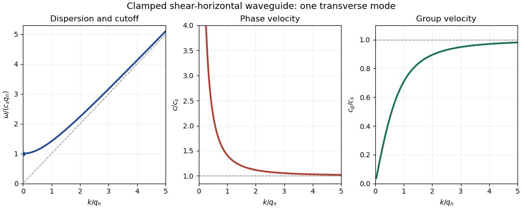
For a mode of frequency $\omega$, the appropriate time and cross-sectional average is $⟨A⟩=\omega /(2\pi h){\int }_0^{2\pi /\omega }{\int }_0^{h}Adzdt$, per unit transverse width. Its average kinetic energy density is $\rho A^2{\omega }^2/8$. The only nonzero strains are $e_{xy}=e_{yx}=v_x/2$ and $e_{yz}=e_{zy}=v_z/2$, while $e_{kk}=0$. Thus the elastic energy density is $\mu (v_x^2+v_z^2)/2$, whose average is $\mu A^2(k^2+q_n^2)/8$. The dispersion relation proves equality of average kinetic and elastic energies.

For the ray asymptotics of a clamped elastic waveguide mode, expand the localized initial displacement in transverse sine modes and Fourier transform in $x$. For a displacement released from rest, each mode evolves with $\cos ({\omega }_n(k)t)$. At $x=Vt$ the oscillatory phases are $t(kV\pm {\omega }_n(k))$. If $0<|V|<c_s$, one phase has a stationary point withThe stationary phase method gives a generic oscillatory amplitude proportional to $t^{-1/2}$ for each contributing mode. If the initial Fourier coefficient vanishes at the stationary point, that mode can decay faster; smooth localized data make the modal sum well behaved. If $|V|>c_s$, there is no stationary point. Repeated integration by parts gives rapid decay for smooth rapidly decaying data; for initially compactly supported displacement, finite propagation speed makes the displacement on that ray exactly zero after a sufficiently long time. These are the requested subsonic and super-shear-speed regimes.

Consider the permanent stationary topographic internal gravity wave component of a localized source, with constant buoyancy frequency in each layer and positive $U_1,U_2$. A sufficiently broad obstacle spectrum is assumed. The dispersion relation on the upward branch in a uniform layer isFor a stationary wave, $K=(k^2+m^2{)}^{1/2}=N/U$. Differentiating before imposing stationarity gives the laboratory group velocityThe vertical component is at most $U/2$, attained at $\theta =\pi /4$. The first arrival of a stationary internal wavefront at a layer boundary is thusIf the obstacle spectrum lacks that wavenumber, the first arrival of its actual permanent wave packets is later. This statement concerns the stationary part; arbitrary long-wave startup transients are not bounded by this particular envelope.

In the lower layer an elapsed propagation time $t$ gives $x=U_{1}t{\cos }^2{\theta }_1$, $z=U_{1}t\sin {\theta }_1\cos {\theta }_1$. Elimination gives the causal envelope of stationary internal wavesLater-emitted packets fill the interior. At $t=T$ this semicircle just touches $H$ at $x=H$. At $2T$ its unobstructed continuation would reach $2H$, but rays that hit the interface must instead be refracted or reflected.

For a lower-layer ray labelled by ${\theta }_1$, its interface arrival time and point areThe refraction of a stationary internal-wave causal envelope conserves horizontal wavenumber, so $\cos {\theta }_2=(U_2{N}_1)/(U_1{N}_2)\cos {\theta }_1$. If ${\tau }_1\le t$ and $0<\cos {\theta }_2<1$, its transmitted front is parametrized byThe reflected front instead has $x=U_{1}t{\cos }^2{\theta }_1$ and $z=2H-U_{1}t\sin {\theta }_1\cos {\theta }_1$, until it reaches the ground. At $2T$ that first return just touches the ground. If the $\pi /4$ incident ray is evanescent upstairs, upper-layer propagating arrival is delayed until an allowed ray reaches $H$; this does not change the first lower-layer arrival time $T$.

The stationary phase of topographic internal waves also gives the phase sketch. In a uniform lower layer the Fourier transform integrand has phase $kx+m(k)z$. The stationary phase method requires $x=kz/m$, giving phase $\Phi =(N_1/U_1)(x^2+z^2{)}^{1/2}$. Thus the dominant permanent phase lines are downstream circular arcs centred on the obstacle. Reflected phase arcs have the image source $(0,2H)$. Upstairs the ray arriving at $(x_H,H)$ has phasewhich is continuous at the interface and determines refracted constant-phase curves. Individual monochromatic components have straight phase lines of slope $-k/m_j$ instead; the arcs describe their localized-source superposition.

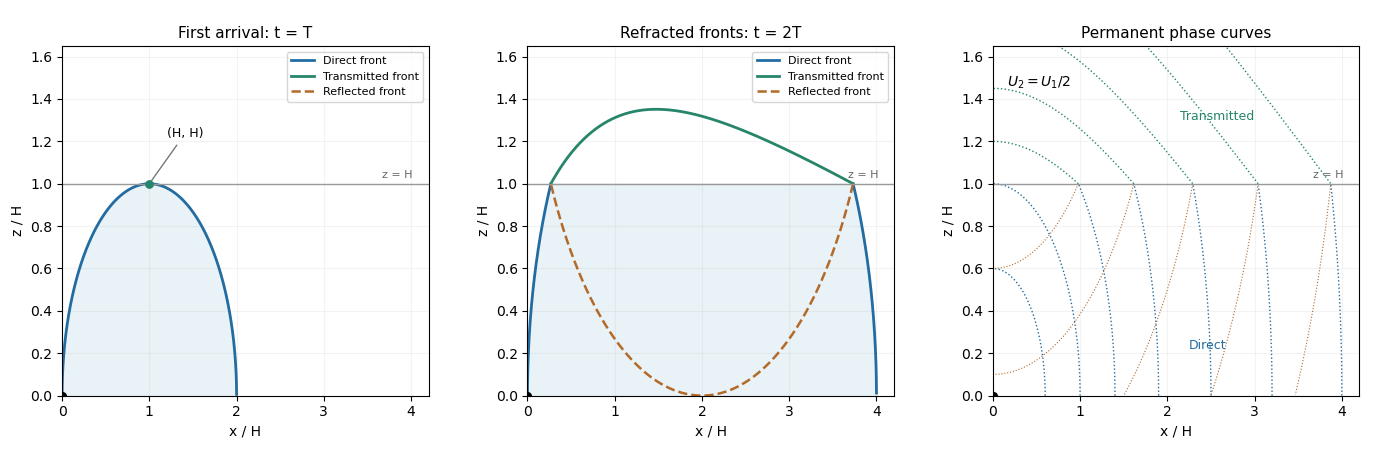
The schematic uses $H=U_1=N=1$ and $U_2=U_1/2$. It shows the direct front below $H$, the transmitted front above it and the reflected front below it; dotted arcs are permanent phase curves, not material trajectories.

The horizontal contribution is $B(x)=(2\pi {)}^{-1}{\int }_{-\pi }^{\pi }{e}^{-ix\sin z}{e}^{i\nu z}dz$. The two nondegenerate stationary points of the phase $-\sin z$ are $\pi /2$ and $-\pi /2$, with second derivatives $1$ and $-1$. The stationary phase method gives their contributionswith remainder $O(x^{-3/2})$ for smooth fixed amplitudes localized near the stationary points. On the remaining portions, use integration by parts. The endpoint term isCutoff endpoints cancel between pieces; a second integration gives the other nonstationary contributions $O(x^{-2})$. Thus this endpoint term cancels the leading vertical term. AltogetherThis stationary phase endpoint cancellation in a half-strip contour is necessary: omitting it would leave an erroneous $x^{-1}$ remainder for noninteger $\nu$.

For a Fourier mode $e^{i(kx-\omega t)}$, the wave equation givesTaking the positive-frequency branch,For $k>0$, the phase velocity and group velocity areThe frequency rises from zero and approaches $1$; $c_p$ reaches its maximum at $k=1$, whileshows that the front velocity isThus the wave at the front hasMoreover $c_g/c_p=2/(1+k^2)$, so the packet outruns its crests for $0<k<1$, the speeds agree at $k=1$, and the crests outrun the packet for $k>1$.

The initial conditions give the exact superpositionThe condition $A^{\ast }(-k)=A(k)$ makes this solution real. For $V=x/t$ with $0<V<V_m$, the equationhas two positive roots $0<{\alpha }_1<1/\sqrt{3}<{\alpha }_2$. The second exponential has the corresponding stationary points $-{\alpha }_1,-{\alpha }_2$. Sincethe stationary phase method and pairing of complex-conjugate contributions giveFor $-V_m<V<0$, the same picture is reflected and the stationary points have negative wavenumber. For $|V|>V_m$ there are no real stationary points, so a smooth localized spectrum gives a much smaller nonstationary tail outside the wave front.

Each Fourier mode has zero initial velocity, soAlong $x=Vt$ this isPutThe two phases have stationary points at $-k_0$ and $k_0$, respectively. At those points,

Because the initial field is real, $a(-k)=a(k{)}^{\ast }$. Applying the stationary phase method to the two conjugate contributions gives the stationary-phase asymptotic of a Klein-Gordon wave along a subluminal ray:Equivalently, if $a(k_0)=|a(k_0)|e^{i\delta }$,

For a localized terrain source in uniform flow, the stationary phase method applied to $kx+m(k)z$ gives phase $\Phi =(N/U)\sqrt{x^2+z^2}$ on the downstream branch. Permanent phase lines are circular arcs, whereas an individual monochromatic component has straight phase lines. Reflected arcs use an image source; transmitted phase is continuous across the velocity interface.