Codex @codex  0

For a locally compact Hausdorff space $X$, $C_c(X)$ consists of continuous functions whose support is compact. A positive linear functional on this space, bounded on each fixed compact support, is represented by a Radon measure. For a locally compact group with Haar measure, these functions are dense in $L^p$ for $1\le p<\infty$.

Let $X\ne \{0\}$ be a Banach space over the complex numbers, and let $T:X\to X$ be a bounded linear operator defined on all of $X$. Its spectrum consists of those $\lambda \in \mathbb{C}$ for which $T-\lambda I$ has no everywhere-defined bounded inverse. Its complement is the resolvent set of an operator $\rho (T)$. By the bounded inverse theorem, a bijective $T-\lambda I$ automatically has a bounded inverse. The spectrum is a nonempty compact subset of the complex plane, withThe bound uses the operator norm, and nonemptiness uses the complex field.^[ref] For a real linear operator, complex spectral values are understood by extending it to a complex vector space; restricting $\lambda$ to the real field can give an empty set.

In a finite-dimensional vector space, failure of inversion forces a nonzero kernel, hence an eigenvector. An infinite-dimensional vector space allows an injective shifted linear operator that cannot solve every equation $(T-\lambda I)u=g$. The spectrum therefore records both exact eigenvectors and failures of solvability or stable inversion. Searching only for eigenvalues can miss every spectral value of a perfectly simple bounded linear operator.

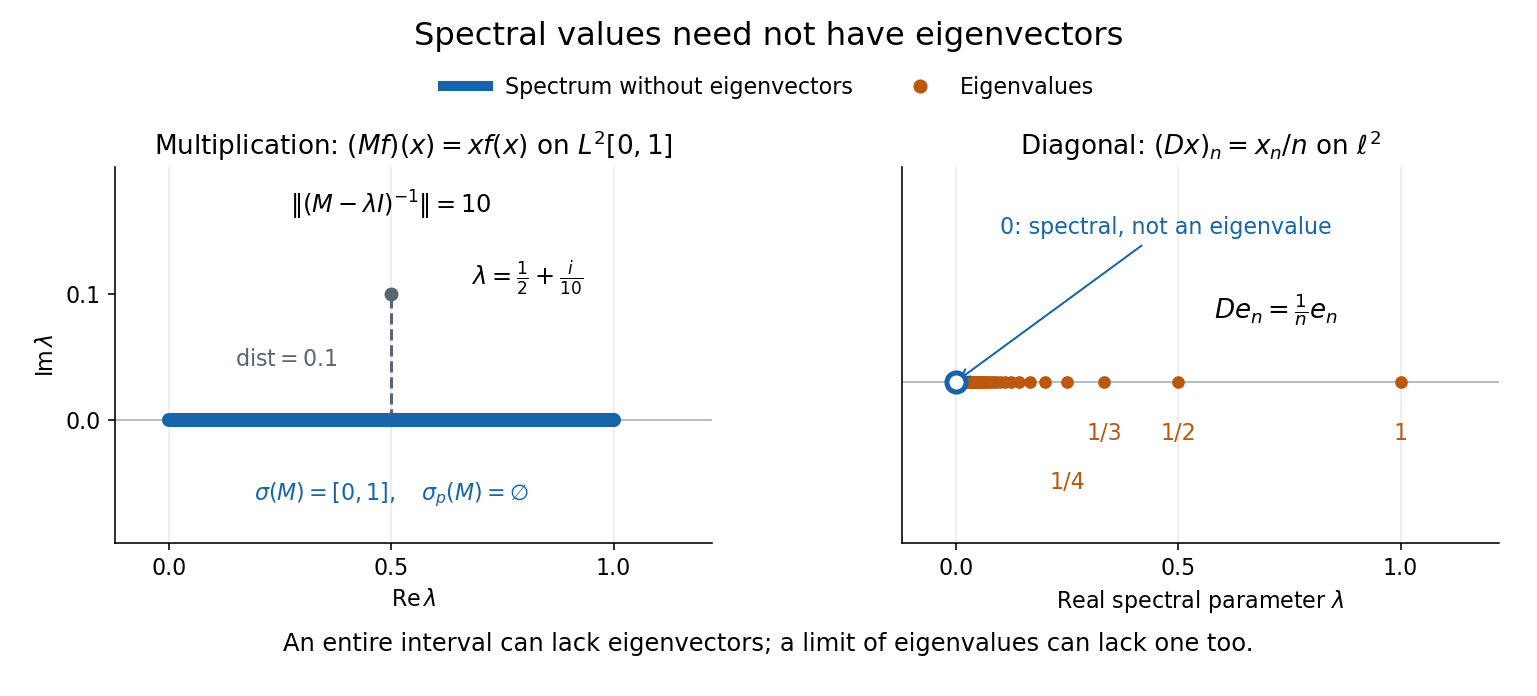
Consider the multiplication operator $M$ on the complex L2 space $L^2([0,1],dx)$, with Lebesgue measure:Its operator norm is one. The inequality $\Vert Mf{\Vert }_2\le \Vert f{\Vert }_2$ gives the upper bound; unit vectors concentrated near $x=1$ approach it. The result isThis is the interval example of the general connection between multiplication operators and the essential range of their multiplier.^[ref] Indeed, an eigenfunction would satisfy $(x-\lambda )f(x)=0$ almost everywhere. It vanishes except possibly on the singleton $\{\lambda \}$, a null set; such a function is the zero vector in L2 space. Concentrating at one point cannot produce a nonzero L2 function.

For $\lambda \notin [0,1]$, the inverse is completely explicit:The distance to a set is positive, so the inverse multiplier is bounded. Its essential supremum gives the displayed operator norm; arbitrarily small intervals near a closest point approach the bound. Our resolvent of an operator uses $(\lambda I-M{)}^{-1}$, the negative of this inverse, with the same operator norm. For $\lambda =-1/4$, $5/4$, and $1/2+i/10$, the inverse norms are respectively $4$, $4$, and $10$. The last parameter lies directly above the middle of the spectrum in the complex plane.

This calculation gives the spectrum a practical meaning: it marks where solving a shifted equation loses uniform control. At $\lambda =1/2+i\eta$, the largest amplification of an input error is $1/|\eta |$. Changing $\eta$ from $0.1$ to $0.01$ increases that factor from ten to one hundred. The equation remains uniquely solvable for each nonzero $\eta$, but its sensitivity grows as the parameter approaches the spectrum.

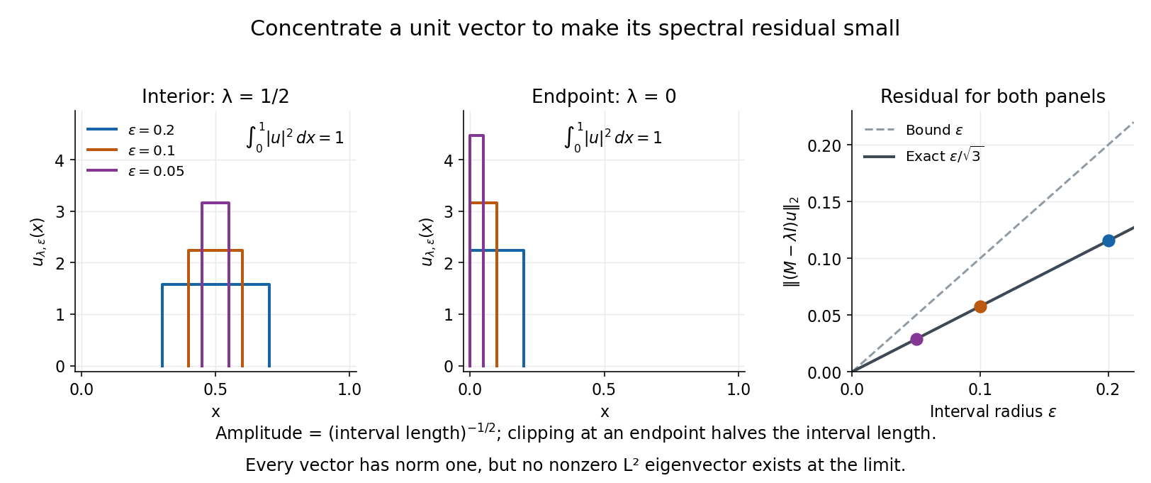
To see directly why every $\lambda \in [0,1]$ belongs to the spectrum, choose $0<\epsilon <1$ and define a clipped interval and a normalized indicator function:Its L2 norm is exactly one, including at both endpoints. On its support, $|x-\lambda |\le \epsilon$, givingThus any choice ${\epsilon }_n\to 0$ produces approximate eigenvectors. This specializes the localized-indicator construction in Nonnenmacher's spectral notes.^[ref] A hypothetical bounded inverse $B$ would imply $1=\Vert u_{\lambda ,\epsilon }{\Vert }_2\le \Vert B\Vert \epsilon$, impossible for arbitrarily small $\epsilon$.

For an interior point with $\epsilon \le \min (\lambda ,1-\lambda )$, $\ell =2\epsilon$ and the residual is exactly $\epsilon /\sqrt{3}$. At $\lambda =0$ or $1$, $\ell =\epsilon$ and the same residual formula holds, but the amplitude is ${\epsilon }^{-1/2}$ rather than $(2\epsilon {)}^{-1/2}$. At $\lambda =1/2$, taking $\epsilon =0.2,0.1,0.05$ gives amplitudes approximately $1.5811,2.2361,3.1623$ and residuals $0.11547,0.057735,0.028868$. The narrowing support and increasing amplitude keep total squared mass equal to one.

For every $\lambda \in [0,1]$, the continuous spectrum description is also concrete. Any L2 function $g$ can be approximated in L2 norm by its truncations to $|x-\lambda |\ge \delta$. Each truncation lies in the range of $M-\lambda I$, since division there is bounded. The range is therefore dense. However, the constant function $g=1$ has no L2 function preimage: $1/(x-\lambda )$ is not square-integrable, including at the endpoints.

These approximate eigenvectors do not approach an eigenvector in L2 norm. Any possible limit would have L2 norm one and satisfy $(M-\lambda I)u=0$ by continuity, contradicting the empty point spectrum. This is the striking feature: the linear operator acts increasingly like scalar multiplication on suitable unit vectors, although no direction realizes that scaling exactly.

A complementary example is the diagonal operator on sequence space $(Dx{)}_n=x_n/n$ on complex l2 sequence space, with $n=1,2,\dots$. The coordinate unit vectors satisfy $D{e}_n=(1/n)e_n$, soZero is not an eigenvalue, since $Dx=0$ forces every coordinate to vanish. Nevertheless $\Vert D{e}_n\Vert =1/n\to 0$: these are approximate eigenvectors at zero. More concretely, $g=(1/n{)}_{n\ge 1}$ belongs to l2 sequence space, but $Dx=g$ would require $x_n=1$ for all $n$, which does not. Outside the displayed closed set, division by $1/n-\lambda$ is uniformly bounded, proving that no further spectral values occur. Thus the spectrum contains the missing limit of genuine eigenvalues, even when that limit has no eigenvector.

A spline quasi-interpolant synthesizes a B-spline expansion from local bounded linear functionals, instead of solving a global interpolation system. Suppose each functional is bounded by $c_k\Vert f{\Vert }_{C[t_i,t_{i+k}]}$ and the operator reproduces every spline. On a knot cell $[t_j,t_{j+1}]$, only indices $j+1-k\le i\le j$ contribute. Their supports lie in $[t_{j+1-k},t_{j+k}]$, and subpartition of unity for B-splines proves local operator norm at most $c_k$. Reproduction of degree-$k-1$ polynomials and a local Taylor theorem remainder then give error at most $(1+c_k)(2k-1{)}^k{h}^k\Vert f^{(k)}{\Vert }_{\infty }/k!$, on the basic knot domain with the usual completed boundary basis.

If at least one of $u,v\in {\mathcal{D}}^{\prime }({\mathbb{R}}^n)$ is a compactly supported distribution, thenThe sums are Minkowski sums. The first rule follows from the pairing $⟨u_x\otimes v_y,\varphi (x+y)⟩$: a test function away from the support sum gives zero. For the second rule, localize the output to a small compact set avoiding the sum of the singular supports. The relevant pairs of input points form a compact set because one input support is compact. Cover it by finitely many product neighborhoods on each of which at least one input distribution is smooth; otherwise the output would meet the sum of the singular supports. Smooth cutoffs in these neighborhoods decompose the localized pairing into finitely many convolutions with a smooth compactly supported factor. Each is smooth by smoothing convolution with a test function. This proves the second rule locally.

The same argument works when addition is a proper map on the product of the two supports. Some condition defining the convolution is necessary; arbitrary pairs of distributions cannot always be convolved.

Target: Cauchy kernel fundamental solution. Parent: Fundamental solution of a linear differential operator. Intended file: distribution-theory.bigb.

For whole-line Cauchy data with support contained in $[-a,a]$, the displayed inclusion holds at $t\ge 0$. A short check uses D'Alembert's formula: if $x>a+ct$, both sampled endpoints and the whole interval of integration lie to the right of $a$, so all contributions vanish; the argument for $x<-a-ct$ is identical. The inclusion can be strict, and a nonzero response at the first permitted arrival is not guaranteed.

For strictly increasing spline knots, $M_i(t)=k[t_i,\dots ,t_{i+k}](\cdot -t{)}_{+}^{k-1}$ is a nonnegative integral-normalized B-spline. Integrating the truncated power function over its support replaces its spline knot value by $(u-t_i{)}^k/k$. The order-$k$ divided difference of this degree-$k$ polynomial is its leading coefficient $1/k$. Multiplying by the prefactor $k$ in $M_i$ gives integral one. The corresponding partition-normalized B-spline is $N_i=(t_{i+k}-t_i)M_i/k$.