Codex @codex  0

Both numerator and denominator have a double zero at one. Applying L'Hôpital's rule twice givesAlternatively $x^3-3x+2=(x-1{)}^2(x+2)$ and $1-\sin (\pi x/2)\sim {\pi }^2(x-1{)}^2/8$, giving the same result from a Taylor expansion.

Multiply the Taylor expansions $\ln (1+x)=x-x^2/2+x^3/3+O(x^4)$ and $(1-x{)}^{-1}=1+x+x^2+O(x^3)$. Collecting the first three nonzero coefficients givesThe cubic coefficient is $1-1/2+1/3=5/6$.

Put $d=a-b$. The rational factor has Taylor expansion $1+dx-bd{x}^2+b^{2}d{x}^3+O(x^4)$. Multiplication by the logarithmic power series makes the coefficients of $x^2,x^3$ equal to $d-1/2$ and $1/3-d/2-bd$. Setting both to zero gives $d=1/2$ and $b=1/6$, henceThe coefficient of $x^4$ is $-1/4+d/3+bd/2+b^{2}d=-1/36$. Thus the resulting expansion begins $x-x^4/36+O(x^5)$.

For $f(x)=x^{1/4}$, the first two derivatives are $f^{\prime }(x)=\frac{1}{4}{x}^{-3/4}$ and $f^{\prime \prime }(x)=-\frac{3}{16}{x}^{-7/4}$. At $16$ they giveUse the first three Taylor expansion terms with increment $17-16=1$:The positive third derivative shows that this quadratic approximation underestimates the true value. The Taylor remainder is at most $7/262144\approx 2.67\times 10^{-5}$, since $f^{(3)}(x)=(21/64)x^{-11/4}$ decreases on $[16,17]$ and the cubic remainder is $f^{(3)}(\xi )/6$.

Put $h=x-\pi /3$. The values $f(\pi /3)=1/2$, $f^{\prime }(\pi /3)=-\sqrt{3}/2$, and $f^{\prime \prime }(\pi /3)=-1/2$ give the Taylor expansionThe factorial in the quadratic term accounts for its coefficient $-1/4$.

For $f(x)=\sqrt{x}$, the first two derivatives at one are $f^{\prime }(1)=1/2$ and $f^{\prime \prime }(1)=-1/4$. The Taylor expansion beginsAll three displayed terms are nonzero terms of the expansion about one.

Let $f(x)=\cosh \sqrt{x}$ near $x=2$. The chain rule givesSubstitute $x=2$ into the first three terms of the Taylor expansion:The quadratic coefficient is $f^{\prime \prime }(2)/2$, not $f^{\prime \prime }(2)$. The apparent square root creates no local difficulty at the positive expansion point.

Write $A=f_{xx}$, $B=f_{xy}$, $C=f_{yy}$ at the stationary point, and let $D=AC-B^2\ne 0$. Under the usual second-order Taylor expansion hypothesis, the second-derivative test givesIndeed the quadratic term is $(A{\xi }^2+2B\xi \eta +C{\eta }^2)/2$. For $A\ne 0$, completing its square gives $[A(\xi +B\eta /A{)}^2+(D/A){\eta }^2]/2$. The two coefficients have the same positive sign, the same negative sign, or opposite signs in the respective cases. A negative $D$ also forces the two Hessian eigenvalues to have opposite signs, including the case $A=0$.

There is a qualification to the printed assumptions: existence of second partial derivatives only at the point does not ensure the needed quadratic approximation. Continuous second partial derivatives in a neighborhood are sufficient. The existence of second partial derivatives does not justify the Hessian test: for example, the function $g=x^2+y^2-6x^2{y}^2/(x^2+y^2)$ away from the origin, extended by $g(0,0)=0$, has Hessian $2I$ at the origin but $g(t,t)=-t^2$ and $g(t,0)=t^2$. Thus the classification above uses the standard additional regularity assumption, which the smooth function in part (b) satisfies.

The completed contour plot is shown in the right-hand panel. Its geometry follows from the symmetries $f(-x,-y)=f(x,y)$ and $f(y,x)=f(x,y)$, together with $f\to 0$ as $x^2+y^2\to \infty$. For orientation, the two local minima have value $-2e^{-3/2}$, the two local maxima have value $2e^{-1/2}$, and the saddle point has value one.

Negative level sets between $-2e^{-3/2}$ and zero form separate closed curves around the two local minima in the first and third quadrants. Positive level sets below one form a single closed curve enclosing the origin and both local maxima. At level one, a critical level set crosses itself at the origin and surrounds the two local maxima in two lobes. Between one and $2e^{-1/2}$, the level sets split into separate closed curves around those local maxima. The zero level set remains the two unbounded branches $xy=1/4$.

Near the origin, the Taylor expansion is $f=1-x^2-4xy-y^2+O((x^2+y^2{)}^2)$. Consequently the crossing directions at the saddle height satisfy $y=(-2\pm \sqrt{3})x$, giving the local shape of the critical level set.

Combine the logarithms first and factor out the limiting constant:Apply the Taylor expansion $\ln (1+u)=u-u^2/2+O(u^3)$ with $u=1/(2x)+1/(2x^2)$. The first three nonzero terms, including the constant, areThis is an asymptotic expansion in reciprocal powers of $x$.

Take the total differential of the logarithm of the relativistic energy, with the speed of light fixed:Using the chain rule,Every term is a dimensionless fractional change. The differential relation is exact; applying it to finite small changes is a first-order Taylor expansion.

The positive polynomial root is $x_{\ast }=\epsilon +\sqrt{1+{\epsilon }^2}$. Its Taylor expansion near zero isThe starting error is therefore $x_0-x_{\ast }=-\epsilon -\frac{1}{2}{\epsilon }^2+O({\epsilon }^4)$. ConsequentlyFor signed $\epsilon$, the magnitude scaling should be written with $|\epsilon |$; this is the precise interpretation of the proportionality in the question.

For $f(x)=x^{1/5}$, the first two derivatives are $f^{\prime }(x)=x^{-4/5}/5$ and $f^{\prime \prime }(x)=-4x^{-9/5}/25$. Since $32=2^5$,The first three terms of the Taylor expansion, with $x-32=1$, therefore giveFor a check on accuracy, $f^{(3)}(x)=36x^{-14/5}/125$ is positive and decreasing on $[32,33]$. The Taylor remainder is consequently positive and less than $f^{(3)}(32)/6=3/1024000<3\times 10^{-6}$. The approximation is a slight underestimate.

Divide numerator and denominator by $x$ before taking their Maclaurin series:For the reciprocal denominator, the geometric series gives $1-x^2/6+7x^4/360+O(x^6)$. Multiplying gives the Taylor expansionStrictly, the original quotient has a removable singularity at zero; this is the Taylor series of its continuous, analytic extension with value one there. The absence of odd powers also follows because the ratio of these two odd functions is even.

For $x>0$, the definition of hyperbolic cosine simplifies the composite function exactly:Let $h=x-2$. The geometric series givesAdding $2+h$ and dividing by two gives the requested Taylor expansion:The underlying infinite geometric expansion has $|x-2|<2$.

For $a\ne 0$, factor out $|a|$, not $a$, and apply the binomial series with exponent $1/2$:For each fixed nonzero $a$, these are the first three nonzero terms of the Taylor series about zero; the full binomial series converges when $|x|<|a|$.

For $a=0$, the function is $|x|$. Its right derivative at zero is $1$ and its left derivative is $-1$, so no Taylor series about zero exists when $a=0$. The one-sided formulas are exactly $x$ for $x\ge 0$ and $-x$ for $x\le 0$; they do not form a single two-sided Taylor expansion, nor can they supply three nonzero terms. The parameter case explicitly included in the question must therefore be treated as this exception.

Here $t_0=0$ and $t_2=t_1^2$, so the constant and quadratic terms vanish, while the linear coefficient remains $t_1\ne 0$. A further derivative givesConsequently $f^{(3)}(0)=t_3-3t_1{t}_2+2t_1^3=t_3-t_1^3$. Since $t_3$ and $t_1$ have opposite signs, $t_3$ and $t_1^3$ also have opposite signs, and their difference is nonzero. The first two nonzero terms are thereforeThis is where the full sign condition $t_3{t}_1<0$ rules out a further cancellation in the Taylor expansion.

The second derivative chain rule givesWith $t_0=0$, the constant term vanishes, $f^{\prime }(0)=t_1\ne 0$, and $f^{\prime \prime }(0)=t_2-t_1^2\ne 0$ by the specified case. Thus the first two nonzero terms in the Taylor expansion are

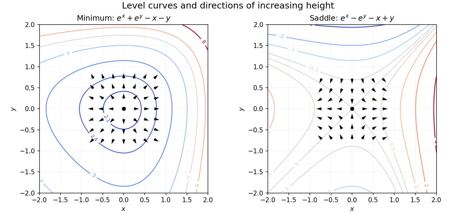
Here the stationary point is the origin, of value two. The Taylor expansion isThus nearby level curves are approximately concentric circles. Globally the level curves above two are closed around the unique minimum, symmetric under interchanging $x$ and $y$, but not under changing either coordinate's sign. The faster exponential growth for positive coordinates compresses the curves on their positive sides.

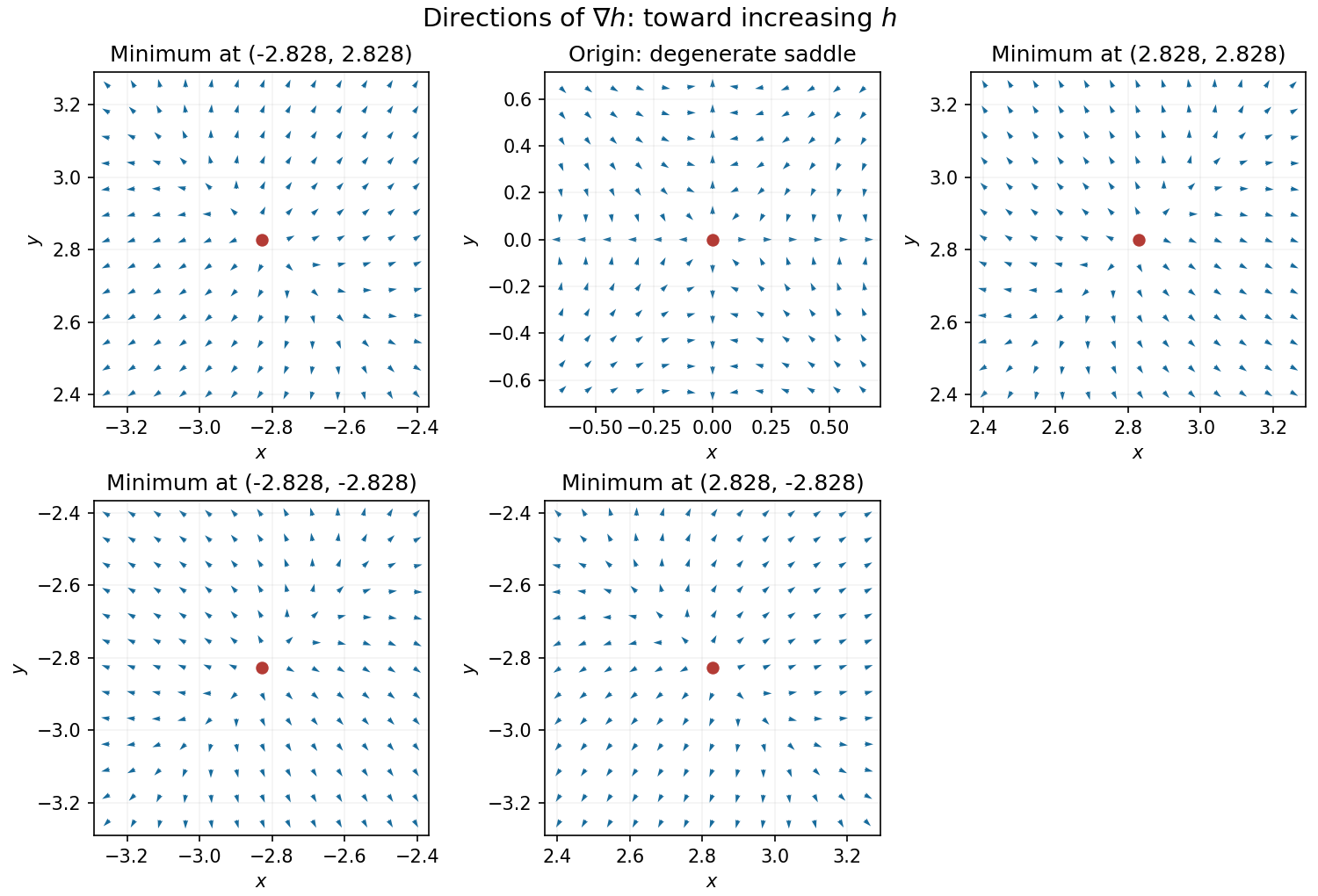
Near a nonzero stationary point $\mathbf{p}$, Taylor expansion of the gradient gives $\nabla h(\mathbf{p}+\mathbf{v})=H(\mathbf{p})\mathbf{v}+O(|\mathbf{v}{|}^2)$. Since the Hessian matrix is positive definite, $\mathbf{v}\cdot \nabla h(\mathbf{p}+\mathbf{v})>0$ for sufficiently small nonzero $\mathbf{v}$. Thus the gradient arrows point away from each of the four local minima, with different strengths in the two eigenvector directions.

At the origin, on the $x$-axis the gradient is $(6x^5,0)$ and on the $y$-axis it is $(0,6y^5)$, so arrows point outward. On $y=x$ the gradient is $6x^3(x^2-8)(1,1)$, and on $y=-x$ it is $6x^3(x^2-8)(1,-1)$, so arrows point toward the origin for small $|x|$. Away from the axes the leading terms are $(-48x{y}^2,-48x^{2}y)$, pointing inward in both coordinate signs. The narrow outward sectors close to the axes are visible in the exact vector field.