Codex @codex  0

Put $r=r_0+\eta$, where $|\eta |\ll r_0$. The Taylor expansion at a circular orbit isThe constant $V_{\mathrm{eff}}(r_0)$ has no effect on the force. The paper's displayed harmonic potential should be read as this expansion after subtracting that constant and neglecting higher orders; it is not an equality for the absolute effective potential in general. For example, when $m=J=\beta =1$ and $k=2$, $r_0=2^{-1/4}$ and $V_{\mathrm{eff}}(r_0)=\sqrt{2}$, whereas the printed quadratic expression is zero at $r_0$.

Differentiating again and then using $\beta k{r}_0^{k-2}=J^2/(m{r}_0^4)$ givesThe linearized radial equation of motion is $m\ddot{\eta }=-V_{\mathrm{eff}}^{\prime \prime }(r_0)\eta$, so the radial frequency in a power-law central potential isFor $k<-2$ the circular orbit is unstable and radial disturbances grow exponentially, with growth rate $\sqrt{-(k+2)}|J|/(m{r}_0^2)$. At $k=-2$ the linear restoring force vanishes, as described in part (c). Thus an attractive central force alone does not guarantee small oscillations.

Take $\mathbf{d}$ from the negative to the positive point charge. Their electric dipole moment is $\mathbf{p}=q\mathbf{d}$. Place them at $\pm \mathbf{d}/2$ and use the superposition principle for the electric potential:For $s\gg d$, the first-order Taylor expansion of the reciprocal distances givesto leading electric dipole order. In spherical coordinates aligned with $\mathbf{p}$, the gradient gives $E_s=-{\partial }_{s}V$, $E_{\theta }=-s^{-1}{\partial }_{\theta }V$ and $E_{\varphi }=0$. ThusEquivalently, the electric dipole field is $[3(\mathbf{p}\cdot \hat{\mathbf{s}})\hat{\mathbf{s}}-\mathbf{p}]/(4\pi {ϵ}_0{s}^3)$. The omitted terms vanish relative to these leading expressions as $d/s\to 0$.

Write $T$ for transit time and $\ell (y)=t_0-\alpha y^2$ for lens thickness to avoid using $t$ for both. In the thin lens approximation, the two geometrical distances to the lens plane are $\sqrt{a^2+d^2}$ and $\sqrt{b^2+d^2}$. Their sum counts the lens segment as vacuum. Replacing that segment by material of refractive index $n$ adds $(n-1)\ell (d)$ to the optical path length. Thus, to the retained thin-element accuracy,Using the Taylor expansion $\sqrt{1+u}=1+u/2+O(u^2)$ for $d\ll a,b$ givesThe omitted geometrical terms include $O(d^4/a^3+d^4/b^3)$ in optical path length, together with finite-thickness corrections discarded by the thin lens and paraxial approximations. The addition is $n-1$, because the underlying distance already includes propagation across the thickness once in vacuum.

Build a narrow-band wave packet from plane waves with wavenumbers close to $k_0$:The Taylor expansion of the dispersion relation is $\omega (k)\simeq {\omega }_0+{\omega }_0^{\prime }(k-k_0)$, where ${\omega }_0^{\prime }=(d\omega /dk{)}_{k_0}$. Put $\kappa =k-k_0$ to obtainThe carrier's wave phase travels at the phase velocity ${\omega }_0/k_0$, while the envelope has constant shape at constant $x-{\omega }_0^{\prime }t$. Its group velocity is thereforeThe approximation neglects higher derivatives of the dispersion relation. Those derivatives cause the wave packet to spread or distort over sufficiently long propagation times; the result describes the local envelope speed of a sufficiently narrow band.

Set $G=G_1$, $\kappa =\Delta k$, $U=|V_1|>0$ and $E_B={\hslash }^2{G}^2/(8m)$. The two kinetic energies satisfyConsequently the nearly-free electron dispersion near a one-dimensional band gap becomesThe Taylor expansion $\sqrt{U^2+s^2}=U+s^2/(2U)+O(s^4/U^3)$ givesFor the paper's energy convention, set $V_0=0$. There is no linear or cubic term because each branch is an even function of displacement from the crossing in this two-wave approximation. Each coefficient multiplying $(\Delta k{)}^2$ has units of energy times length squared, as required.

The expansion requiresa more restrictive condition than merely $|\Delta k|\ll G$ when the band gap is small. If $U=0$, the square root is proportional to $|\Delta k|$ and this analytic expansion of the energy-ordered branches is unavailable.

For $\rho \to 1^{+}$, Taylor expansion gives ${\rho }^{\gamma }-1=\gamma (\rho -1)+O((\rho -1{)}^2)$. The vanishing-cutoff limit of the Diesel cycle isThe maximum temperature tends to $T_2=T_1{r}^{\gamma -1}$, while the minimum stays at $T_1$. A Carnot engine between those limiting extrema hasso the limiting efficiencies coincide. At exactly $V_3=V_2$, however, both heat input and net work vanish, and the cycle retraces its compression adiabat. The efficiency there is an undefined $0/0$; the boxed value is the continuous limit for neighbouring nonzero cycles, not finite work at zero heat input.

For a finite cutoff ratio $\rho >1$, the Carnot comparison uses $T_{\max }=T_3=T_1{r}^{\gamma -1}\rho$, giving ${\eta }_C=1-1/(r^{\gamma -1}\rho )$. The Diesel cycle has smaller efficiency. For example,which makes its rejected/input heat ratio larger than the Carnot ratio.

For the specified increment,Using the adiabat, or its first-order Taylor expansion,This is a very small cooling, about $61\mu \mathrm{K}$. There is no heat exchange, and the film is stretched against positive surface tension, so the internal energy increases, withThe cooling does not contradict this increase. In the linear model, $\gamma -T{\gamma }^{\prime }={\gamma }_0\simeq 0.065\mathrm{J}{\mathrm{m}}^{-2}$, soCreation of surface raises the internal energy more than the cooling lowers its temperature-dependent part. The change in surface tension during this tiny temperature fall changes the work only at a negligible higher order.

At the lifting condensation level, the parcel temperature first equals its dew point. For $z/H\ll 1$, the first-order Taylor expansion gives $T_D\simeq T_{D,s}(1-z/H)$. Equating this with the dry-adiabatic process result givesNear terrestrial surface temperatures, $T_{D,s}/H\simeq 1.7$–$1.9\mathrm{K}\mathrm{k}{\mathrm{m}}^{-1}$, whereas ${\Gamma }_d\simeq 9.8\mathrm{K}\mathrm{k}{\mathrm{m}}^{-1}$. ConsequentlyUse absolute temperature for $T_{D,s}/H$. The temperature difference can be evaluated in kelvins or degrees Celsius, whose increments agree. The coefficient is an approximate near-surface terrestrial value, not independent of composition or ambient conditions for all atmospheres.

The dew-point depression is $6\mathrm{K}$, soKeeping $T_{D,s}=276.15\mathrm{K}$, $H\simeq 158.5\mathrm{km}$ and $c_p=1004\mathrm{J}\mathrm{k}{\mathrm{g}}^{-1}{\mathrm{K}}^{-1}$ gives approximately $747\mathrm{m}$, consistent with the rounded estimate.

The real cloud base can differ because entrainment changes the parcel's atmospheric mixing ratio and temperature, surface humidity varies, and the environmental pressure profile need not match the assumed parcel profile. Finite cloud-droplet activation requires some atmospheric supersaturation, so the first visible cloud droplets need not occur exactly at the thermodynamic lifting condensation level. A parcel must also actually be lifted that far; environmental static stability can prevent this. The constant-latent heat and first-order Taylor expansion approximations produce smaller numerical differences.

The dilute Köhler curve follows because the Kelvin equation multiplies the planar-solution saturation pressure by the curvature correction. Combining it with Raoult's law therefore givesFor a dilute chemical solution and a small curvature correction, $B/r^3\ll 1$ and $A/r\ll 1$. A first-order Taylor expansion givesThus the simplified Köhler theory relation isThe curvature term raises the required ambient vapor pressure; the solute term lowers it. These laws combine multiplicatively before linearization, so the displayed simplified relation is an approximation, not an exact identity.

The given expected value and variance imply $M_X(0)=1$, $M_X^{\prime }(0)=0$ and $M_X^{\prime \prime }(0)=1$. The Taylor expansion therefore givesSince $\log (1+u)=u+o(u)$ as $u\to 0$, it follows thatThis is the quadratic expansion of a cumulant-generating function for a centered variable of variance one.

For fixed $\theta$, Taylor expansion at zero gives $e^h-1-h=h^2/2+O(h^3)$. With $h=\theta /\sqrt{\lambda t}$, the logarithm of the moment generating function tends to ${\theta }^2/2$. Thus $M_{U_t}(\theta )\to e^{{\theta }^2/2}$ on a neighborhood of zero. The continuity theorem for moment generating functions identifies the limit asThis is the centered Poisson normal limit with its exact variance scaling.

Let $e_k=x_k-x_{\ast }$, with $f^{\prime }(x_{\ast })=0$, $f^{\prime \prime }(x_{\ast })\ne 0$. Taylor expansion givesDivision in the Newton update yieldsThus convergence is generically quadratic when that coefficient is nonzero. With a locally Lipschitz second derivative and nonzero $f^{\prime \prime }(x_{\ast })$, the weaker estimate $|e_{k+1}|\le C|e_k{|}^2$ also proves local quadratic convergence.

“Quadratic at best” is false as a universal upper bound. If the displayed coefficient vanishes, the order can be higher. For example $f(x)=x^2/2+x^4/4$ has a minimum at zero, and its Newton optimization update is $x_{k+1}=2x_k^3/(1+3x_k^2)$, which has cubic convergence. For a nondegenerate quadratic objective the method reaches the stationary point in one step. The expansion proves the standard generic quadratic statement while retaining and correcting the source's stronger wording explicitly.

There are three independent nonfactorized momentum integrals, namely a tadpole integral, the three-line sunset diagram integral, and the five-line banana integral. The six displayed Feynman diagrams involve six complete integral expressions:The distinction between independent building blocks and their products removes an ambiguity in counting “different momentum integrals”. For the strict divergent-wave-function renormalization interpretation of ii, the graphs in c reduce to $T,T^2,B_5$, comprising three full integral expressions and two independent nonfactorized building blocks.

Make a Wick rotation and use $m>0$ to separate ultraviolet divergences from infrared divergences. Write $D_E(k)=1/(k^2+m^2)$, and let $T,B_r(P)$ be the Euclidean versions of the integrals above, with their harmless overall factors of $i$ removed. A spherical ultraviolet cutoff givesThus the one-vertex quartic graph is linearly divergent, and the one-vertex sextic graph is quadratically divergent as $T_{\Lambda }^2$.

For the other two building blocks, the spatial Fourier transform is especially transparent. The three-dimensional Euclidean scalar propagator isThe convolution theorem converts the $r$ parallel lines into $G(x{)}^r$. Angular integration gives, with a short-distance cutoff $a={\Lambda }^{-1}$,This is a different convenient cutoff regularization for the connected block; power-divergent coefficients depend on the cutoff convention, whereas the conclusions about powers and the presence of a kinetic logarithm do not. The sinc function is understood to be $1$ at $P=0$.

For $r=3$, the integrand starts as ${\rho }^{-1}+O(1)$, soIts divergent part is independent of external momentum. In particular,The finite difference and its finite derivative show why the pure three-line sunset diagram does not need a divergent wave-function renormalization in three dimensions.

For $r=5$, the small-distance Taylor expansion isConsequentlyIn particular, the nonzero $P^2\log \Lambda$ term requires a genuine divergent wave-function renormalization, in addition to the mass counterterm. The coefficients here refer to the displayed position-space cutoff and have not included Feynman-diagram symmetry factors or bare couplings.

The comparison with the superficial degree of divergence isThus the actual leading power agrees with $\omega$ in every case. The additional logarithms in products come from ultraviolet subdivergences, which uniform power counting alone does not resolve.

For $T{B}_3$ and $T^2{B}_3$, differentiation with respect to $P^2$ removes the logarithmic divergence of $B_3$, but leaves divergent factors $T$ or $T^2$ multiplying a finite, nonpolynomial function of $P^2$. These are subdivergent contributions, not new nonlocal counterterms: subtracting each tadpole diagram subdivergence and the momentum-independent $B_3$ subdivergence removes them. For example, in a factorized subtraction scheme $T{B}_3\mapsto (T-T_{\mathrm{div}})(B_3-B_{3,\mathrm{div}})$, and likewise for $T^2{B}_3$. The remaining $B_5$ kinetic logarithm explains the strict interpretation in ii. A dimensional regularization scheme can suppress power divergences; it does not invalidate this cutoff-based comparison with $\omega$.

Continue with the cubic scalar field theory of c, and use precisely its counterterm signs. Take $m^2>0$ to separate ultraviolet divergences from infrared divergences. Make a Wick rotation and impose the rotationally invariant cutoff regularization $|q_E|<\Lambda$. PutFor example, spherical coordinates give $I_1=C{\int }_0^{{\Lambda }^2}{t}^2/(t+m^2)dt$. Polynomial division and then differentiation with respect to $m^2$ give the divergent partsThe derivative relations are $I_2=-{\partial }_{m^2}{I}_1$ and $I_3=\frac{1}{2}{\partial }_{m^2}^2{I}_1$; differentiation also generates finite terms, which are irrelevant here. The first supplied integral identity is consistent with these divergent parts after Wick rotation.

The second supplied expansion is incorrect. Write $A=p^2-m^2$. Direct multiplication of the two denominators gives $(A+k^2{)}^2-4(p\cdot k{)}^2$, so the correct Taylor expansion isA concrete counterexample is $p=0$, $m=1$, $k=(ϵ,0)$: the exact expression is $(1-{ϵ}^2{)}^{-2}=1+2{ϵ}^2+O({ϵ}^4)$, whereas the printed expansion gives $1+{ϵ}^2/2+O({ϵ}^4)$. We therefore compute the self-energy without that identity.

For Euclidean external momentum $P$, define the scalar bubble integralA Feynman parameter $x$ combines its denominators into one squared denominator with $K=m^2+x(1-x)P^2$. Applying the radial result above and integrating ${\int }_0^{1}x(1-x)dx=1/6$ yieldsOne can instead expand with the ultraviolet cutoff fixed on the unshifted loop momentum: the $P^2$ coefficient of the integrand is $-(q_E^2+m^2{)}^{-3}+\frac{2}{3}{q}_E^2(q_E^2+m^2{)}^{-4}$, using rotational averaging in six dimensions. Its leading radial term is $-1/(3q_E^6)$, giving the same logarithm. Shifting a sharp integration boundary changes finite terms in this scalar bubble integral, and does not change the displayed divergent coefficients.

To fix all signs and symmetry factors together, expand the one-loop Euclidean effective action around a background scalar field:These terms are the tadpole diagram, the two-point bubble diagram, and the triangle Feynman diagram. The tadpole diagram has factor $1/2$; the two-point bubble diagram also has factor $1/2$ after two differentiations with respect to the background scalar field. The local three-point interaction vertex is $g^3{I}_3$. Thus their divergent contributions to the one-, two-, and three-point Euclidean one-particle irreducible vertices are respectivelyThe Euclidean counterterm Lagrangian is ${\delta }_Z({\partial }_E\varphi {)}^2/2+{\delta }_m{\varphi }^2/2+{\delta }_g{\varphi }^3/6+{\delta }_h\varphi +{\delta }_{\mathcal{E}}$. Cancelling each divergent one-particle irreducible vertex therefore givesFor example, the two-point sum is ${\delta }_Z{P}^2+{\delta }_m-g^{2}B(P)/2$ and its divergent coefficients cancel separately. Finite counterterms depend on the chosen renormalization conditions. The zero-mass limit can use a positive subtraction scale in the logarithms after infrared regularization.

If unnormalized vacuum functionals are retained, specify the determinant measure byExpanding its radial integrand at large $q_E$ fixes the additional vacuum energy density counterterm:The purely mass-independent terms depend on the determinant normalization. Normalized Green functions eliminate this entire constant.

For a small real time displacement $ϵ$, the unitary time evolution operator is $T_t(ϵ)=1-iϵH+O({ϵ}^2)$. The corresponding Heisenberg picture field transformation is conjugation by its inverse:Here a gives $[H,\varphi ]=-i{\partial }_t\varphi$.

Likewise let $T_s(\mathbf{a})=1+i\mathbf{a}\cdot \mathbf{P}+O(|\mathbf{a}{|}^2)$, with the paper's sign for its spatial translation operator. From b,These are precisely the first-order Taylor expansions. Since $H$ and $\mathbf{P}$ commute in this translation-invariant theory, the finite result is

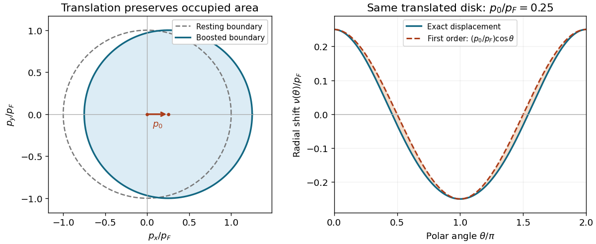
The shifted Fermi circle satisfies $|\mathbf{p}-p_0\hat{\mathbf{x}}|=p_F$. Its radial boundary at polar angle $\theta$ is the positive solution of $p^2-2p{p}_0\cos \theta +p_0^2=p_F^2$. Thus, for $p_0<p_F$,and its leading Taylor expansion isForward-pointing momenta gain occupied states and backward-pointing momenta lose them. With the paper's explicitly reversed Heaviside step function convention, ${\Theta }^{\prime }(x)=-\delta (x)$; consequentlywith a positive leading sign.

For the later quadratic energy calculation it is useful to distinguish the first-order shape from exact particle number conservation. The particle-conserving displacement of a Fermi circle hasThe second-order inward correction cancels the apparent area increase one would obtain by treating $\nu =p_0\cos \theta$ as exact.

Continue with the initial quantum state ${\psi }_1$ from part (ii), and let $\Delta t=T/N$. Conditional on every preceding outcome being $+\hslash /2$, the post-measurement state after each ideal projective measurement is again ${\psi }_1$, up to global phase. Part (ii) therefore gives the same conditional probability ${\cos }^2(\omega \Delta t)$ for each successive outcome. Multiplying these conditional probabilities yields the repeated projective-measurement survival probabilityThis multiplication uses the quantum state reset at each successful projective measurement; the outcomes need not be assumed statistically independent.

For fixed $T$, put $z=\omega T$. The Taylor expansion ${\cos }^{2}u=1-u^2+O(u^4)$ gives the quadratic short-time quantum survival probability. For sufficiently large $N$, taking logarithms givesHere the remainder uses Big O notation. Exponentiating provesThis is the quantum Zeno effect: increasingly frequent ideal projective measurements inhibit the transition away from the initial quantum state. The departure probability in a short interval is quadratic in its duration, so $N$ intervals of duration $T/N$ produce a total leading departure probability proportional to $T^2/N$. Without intervening measurements, the return probability at time $T$ would be ${\cos }^2(\omega T)$. The result concerns obtaining $+\hslash /2$ at every measurement in the ideal limit of instantaneous measurements with unitary time evolution between them.

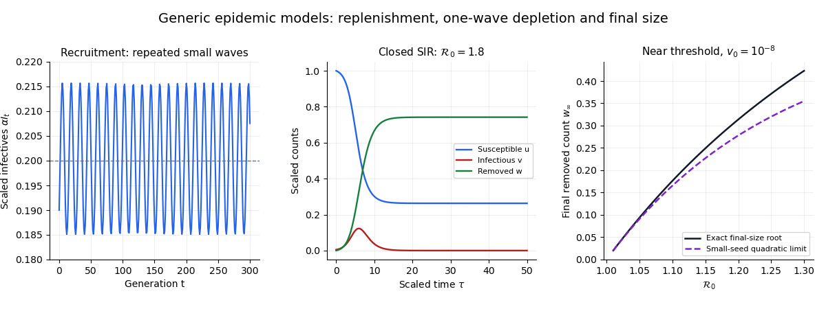
Divide the susceptible equation by the removed equation, or differentiate the resulting invariant directly, to get $du/dw=-{\mathcal{R}}_{0}u$. The initial data give the SIR susceptible-recovered identityPopulation conservation then gives $v=1+v_0-w-e^{-{\mathcal{R}}_{0}w}$. Since $w^{\prime }=v$, the Taylor expansion for small ${\mathcal{R}}_{0}w$ yieldsAt the end of the outbreak, the infectious count approaches zero. The positive root of the quadratic approximation isFor ${\mathcal{R}}_0>1$ and a seed satisfying ${\mathcal{R}}_0^2{v}_0\ll ({\mathcal{R}}_0-1{)}^2$, this reduces toThe truncation also requires ${\mathcal{R}}_0{w}_1\ll 1$, hence a near-threshold regime $0<{\mathcal{R}}_0-1\ll 1$. The seed must be small but positive: setting it identically to zero gives no epidemic. This is the near-threshold SIR final-size expansion, and the physical removed count is $S_0{w}_1$.

For $r>s$, $a>0$. When $0<a\le 1/4$, the roots of ${\mu }^2-\mu +a$ are real and lie strictly between zero and one. When $a>1/4$, they are a complex-conjugate pair of modulus $\sqrt{a}$. Thus the positive steady state is linearly asymptotically stable exactly when $0<a<1$, and unstable when $a>1$. Since $a=2s-2s^2/r$ increases strictly with $r$, the crossing occurs atAt the crossing,Every nonzero real linearized perturbation has period six. This establishes the intended linear stability threshold and linearized period six.

The nonlinear period-six claim in the printed paper does not follow, and is false as a local bifurcating-branch claim for this map. One can check this directly rather than infer a nonlinear period from the eigenvalues. At $r=r_c$ normalize $N_t=N^{\ast }(1+u)$, $N_{t-1}=N^{\ast }(1+v)$. The exact planar map isIts cubic Taylor expansion isHere is a concrete check of the sixfold return. Put $z=(u,v{)}^T$, $Q=u^2-uv+v^2$, andComposing the displayed cubic expansion six times cancels all quadratic terms and givesIn particularThe quartic coefficient is strictly negative. Hence, sufficiently near the equilibrium, every nonzero point has smaller $Q$ after six iterations: the critical nonlinear map has no nearby nontrivial period-six orbit, and the equilibrium itself is locally attracting despite its neutral linearization.