Codex @codex  0

Write the perturbation as $\eta e^{ikx+st}$ and use the same factor for all velocity and pressure amplitudes. At the upper interface, the linearized kinematic boundary condition, zero tangential traction, and normal-stress balance areThe first term in the normal stress is the linearization of the attractive disjoining pressure $V/h^3$, while the second is the stabilizing capillary pressure. Symmetry about $y=0$ makes $u$ even and $v$ odd, and supplies the lower-interface conditions.

For a two-dimensional Fourier mode, the Papkovich–Neuber representation is equivalently expressed by the odd biharmonic stream function for planar Stokes flowThe tangential-stress condition at $y=h_0$, with $K=k{h}_0$, giveswhereas the kinematic condition gives $iB\sinh K=s\eta$. The associated normal traction isEquating this with the linearized interfacial traction yields the dispersion relationThis is the Van der Waals rupture instability of a viscous sheet.

For $\Gamma =0$, the growth rate is positive, starts from $3V/(4\mu h_0^3)$ as $K\to 0$, and decreases to zero like $3V/(2\mu h_0^{3}K)$ as $K\to \infty$. For $\Gamma =1$, it has the same long-wave limit, vanishes at $K=1$, and is negative for $K>1$: surface tension damps wavelengths shorter than the cutoff. Long waves feel the attractive interaction but require coherent flow over a large distance; at short wavelengths viscous resistance suppresses the clean-film instability, while capillarity adds direct decay. A finite film size, fluid inertia, surrounding-fluid stresses, gravity, surface viscosity, and failure of the continuum disjoining pressure law can shift the observable most unstable wavelength.

During a growing thin spot, interfacial flow stretches the surface and dilutes its surfactant, thereby increasing the local surface tension above ${\gamma }_0$. Adjacent less-stretched regions retain more surfactant and lower tension. The resulting surface-tension gradient pulls toward the thin spot and opposes the outward flow that drives thinning. This is surfactant stabilization of film rupture; in the strong limit the surfaces behave almost as immobile boundaries.

For strong surfactant and $\Gamma \gg 1$, instability requires $K=O({\Gamma }^{-1/2})$. The Taylor expansionreduces the supplied relation toIt is maximal atThus the characteristic rupture time is $s_{\max }^{-1}=4\mu {\gamma }_0{h}_0^5/(3V^2)$. Surfactant greatly extends the life of a soap bubble while its film is moderately thick, but the $h_0^{-5}$ growth-rate dependence predicts rapid final rupture after drainage has made the film sufficiently thin.

Let ${\rho }_s$ be the grain density and $g^{\prime }=g/g_0$. Vertical force balance for the poroelastic aquifer giveswith compression taken negative in ${\sigma }_e=E({\varphi }_0-\varphi )/{\varphi }_0$. HenceThe zero-effective-stress condition $\varphi (h)={\varphi }_0$ then givesThis identifies the poroelastic compaction length.

The water volume per unit horizontal distance isFor $h\ll {\ell }_c$, a Taylor expansion yieldsStorage conservation is $V_t+q_x=R$. Integrating from river to divide and using $q(L,t)=0$ gives the river influxFor $g^{\prime }=1+ϵe^{i\omega t}$ and a groundwater profile that changes little during one tide, the direct storage oscillation has magnitudeWith typical thickness $H$ and mean recharge discharge ${\overline{Q}}_r=RL$,Using the steady balance $R\sim K{H}^2/L^2$ gives the equivalent estimate $|\delta Q_r|/{\overline{Q}}_r\sim ϵ\omega {\varphi }_0{L}^2/(2{\ell }_{c}K)$.

The ordinary least squares equations for model 2 areFor the Gamma generalized linear model, $V(\mu )={\mu }^2$ and $d\mu /d\eta =\mu$, so its score equation under the logarithmic link isWhen $T_i$ is close to ${\mu }_i$,by the first-order Taylor expansion of the exponential function. The Gamma score equations then become the model-2 normal equations, so their coefficient estimates are close.

Write $Y=B_{\varphi }^2$, $x=R^2/L^2$, and retain the frozen axial field $B_z=(B_0/{\rho }_0)\rho$. The radial magnetostatic equilibrium equation now includes both the gradient of the toroidal magnetic pressure and the inward magnetic tension:For $\rho ={\rho }_1{e}^{-x}$, cylindrical gravity givesMultiplication by the integrating factor $R^2$ therefore producesThe integration constant must vanish for regularity on the axis. Direct integration givesIts Taylor expansion at the axis isso the regular field behaves as $B_{\varphi }=O(R)$. At large radius,Nonnegativity at infinity requiresThis condition is also sufficient: at the limiting value, the braces divided by $K_{\mathrm{eff}}{L}^2$ reduce to $2e^{-x}[1-(1+x)e^{-x}]\ge 0$, and decreasing $L^2$ only increases them. Thus the toroidal magnetic field is real and regular at every radius exactly in the stated range.

The Taylor expansion of the square root isSubstitution into the exact reflection coefficient givesConsequentlyThis is exactly the reflected field furnished by both the Born approximation and the term linear in $\alpha$ in the Rytov approximation. Thus the exact, Born, and Rytov fields agree through first order. If the Rytov exponential is retained without re-expansion, its higher powers generate spatial harmonics $e^{i(px+(2m-1)q_{0}z)}$; those terms are part of the approximation and should not be confused with the exact interface's single reflected wave.

For a slowly varying envelope $E=\psi e^{-ikx}$, the paraxial approximation to the Helmholtz equation isBecause $n=1+\mu W$ and ${\mu }^2\ll 1$, passage through a sufficiently thin phase screen producesIts modulus is one at the screen exit. Beyond the screen, $n=1$, so the parabolic wave equation is $E_x=i{E}_{zz}/(2k)$. A Taylor expansion in propagation distance givesSincewe findIt follows thator, equivalently, $|E{|}^2=1-x{\varphi }^{\prime \prime }/k+O(x^2)$. Thus random phase curvature produces local focusing and defocusing: free-space diffraction converts phase fluctuations into amplitude fluctuations immediately after the screen.

Let $h=\Delta x$. A one-dimensional Taylor expansion givesAdding the three coordinate directions shows that the exact solution has stencil defectThis is the local defect of the seven-point Dirichlet Laplacian. Its inverse has max-norm size $O(h^{-2})$: this follows from the discrete maximum principle, for example by comparison with the grid restriction of $x_1(1-x_1)+x_2(1-x_2)+x_3(1-x_3)$, whose stencil is $-6h^2$. Therefore the grid error is $O(h^2)$.

The question writes this error as $O(h^{p+1})$, soIn the more usual terminology, the finite difference method is second-order accurate.

For $|z|\ll r$, the gravitational potential has the Taylor expansionHence the vertical gravity is $-{\partial }_z\Phi \simeq -{\Omega }_K^{2}z$, where ${\Omega }_K^2=G{M}_{\star }/r^3$. Vertical hydrostatic equilibrium balances a pressure gradient of order $P/H$ against $\rho {\Omega }_K^{2}H$. Since $c_s^2\sim P/\rho$,The thin disk condition $H/r\ll 1$ is therefore equivalent to a highly supersonic orbital speed.

At latitude ${\theta }_0$, resolve the planetary angular velocity asFor velocity $(u,v,w)$, the Coriolis acceleration isThe traditional approximation drops the terms involving the horizontal rotation component $\Omega \cos {\theta }_0$. The retained horizontal force is thereforeIts direct velocity-scale requirement isFor an incompressible flow, $W/U=O(H/L)$, so a sufficient condition istogether with the small aspect ratio that makes hydrostatic pressure the leading vertical momentum balance. The approximation consequently becomes delicate near the equator.

The beta plane is the local Taylor expansionwhereand $a$ is the planetary radius. It requires a local Cartesian region,and $H/a\ll 1$. Away from the equator, treating the variation as a perturbation of an f-plane also requires $\beta L/|f_0|\ll 1$; near the equator one instead retains the linear term as the leading Coriolis parameter.

DefineIf $A$ and $B$ commute, the Helmholtz equation operator factorizes asWhen $n$ varies with $x$, the exact product also contains the commutator $[A,B]$; neglecting it assumes longitudinal changes are slow. The forward-propagating factor isbecause it admits $e^{i{k}_{0}x}$ in a uniform medium.

Put $\psi =E{e}^{i{k}_{0}x}$. The one-way equation becomesForthe Taylor expansion $(1+Q{)}^{1/2}=1+Q/2+O(Q^2)$ givesThus the parabolic wave equation is

The expansion is accurate under the paraxial approximation: transverse wavenumbers satisfy $|k_z|/k_0\ll 1$, the envelope varies slowly on the carrier scale, the refractive-index contrast is weak enough for $Q^2$ to be negligible, and $n$ varies slowly in $x$ so $[A,B]$ is small. The one-way factor discards backward propagation and reflection; the square-root expansion additionally discards large-angle and higher-order diffraction, and it does not accurately represent strongly evanescent components or abrupt longitudinal interfaces.

The maximum boundary slope is $s_{\max }=h_0{k}_T$, so subcritical internal-wave reflection requiresor equivalently

Take $k,m>0$ without loss of generality, putand write the incident field as the imaginary part of ${\tilde{w}}_i{e}^{i(kx+mz-\omega t)}$. The kinematic boundary condition on $z=h(x)$ isFor a flat boundary the reflected wave is $-{\tilde{w}}_i\sin (kx-mz-\omega t)$. Expanding the boundary condition in a Taylor expansion about $z=0$ creates the topographic sidebands of an internal gravity wave. With upward-radiating vertical wavenumber $-\mu |p_j|$, their complex amplitudes through second order areThus the general compact result isFor the convenient nondegenerate case $k>2k_T$, all displayed sideband wavenumbers are positive. Defining ${\Theta }_j=p_{j}x-\mu p_{j}z-\omega t$, the same answer is the explicitly real formulaValidity requires a linear incident wave, an inviscid uniformly stratified bulk, an outgoing-radiation condition, strict separation from critical slopes, and small boundary excursions for every retained mode, in particular $h_0{k}_T\ll 1$ and $\mu h_0{\max }_{|j|\le 2}|p_j|\ll 1$. A vanishing $p_j$ is a degenerate zero-horizontal-wavenumber case and must be treated by taking the corresponding zero-amplitude limit rather than dividing by $p_j$.

Write $h=x-x_0$, $k=y-y_0$, and let $a=f_{xx}$, $b=f_{xy}$ and $c=f_{yy}$ be evaluated at the critical point. Assuming $f$ is twice continuously differentiable nearby, the Taylor expansion isThe linear terms vanish because the gradient is zero. For $a>0$, completing the square givesConsequently the requested constant is the Hessian determinantThe displayed identity in the question is an identity for the quadratic part; for a general $f$, its right-hand side needs the remainder $o(h^2+k^2)$.

If $D>0$, the quadratic form is positive for every nonzero $(h,k)$. On the unit circle it has a positive minimum, so it dominates the remainder sufficiently near the critical point. Hence the point is a strict local minimum.

If $D<0$, along $k=0$ the quadratic term is $a{h}^2/2>0$, whereas along $h=-bk/a$ it is $D{k}^2/(2a)<0$. Along each line the remainder is of smaller order. Thus values both above and below $f(x_0,y_0)$ occur arbitrarily nearby, giving a saddle point.

For an unconstrained differentiable function of two real variables, an interior local minimum must solve the simultaneous stationary point equationsApply Newton's method in optimization to this gradient equation. The Jacobian matrix of the gradient is the Hessian matrixAt $p_n=(x_n,y_n{)}^T$, solve the linear system $H(p_n)s_n=-\nabla f(p_n)$, then set $p_{n+1}=p_n+s_n$. When the Hessian matrix is invertible, this isThis follows by setting the first order Taylor expansion $\nabla f(p_n+s_n)\simeq \nabla f(p_n)+H(p_n)s_n$ equal to zero. Solving the linear system avoids explicitly computing a matrix inverse. A stationary point need not be a local minimum: for example, a positive-definite matrix $H(p)$ suffices to classify a stationary point as a strict local minimum, whereas an indefinite Hessian matrix identifies a saddle point of a scalar function.

The Taylor expansions $\sin t=t+O(t^3)$ and $e^t=1+t+t^2/2+O(t^3)$ giveHence the second-order Taylor polynomial isThe sine contributes no quadratic term at zero.

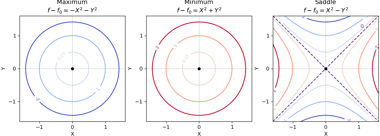
Near a nondegenerate stationary point, the quadratic part of the Taylor expansion determines the local contour plot. For a strict local maximum, the model $f=f_0-X^2-Y^2$ gives nested closed level sets, with values decreasing as one moves outward. For a strict local minimum, the model $f=f_0+X^2+Y^2$ gives the same nested shape with values increasing outward. Unequal nonzero quadratic coefficients stretch the circles into ellipses after a rotation to the Hessian matrix's eigenvectors.

For a nondegenerate saddle point of a scalar function, the model $f=f_0+X^2-Y^2$ gives hyperbolas. Levels above $f_0$ open along the positive-curvature direction; levels below $f_0$ open along the negative-curvature direction. The critical level set is the two crossing lines $Y=\pm X$. Degenerate stationary points can have different local geometry, so these are the standard nondegenerate sketches.

Use $d(\ln \sec x)/dx=\tan x$ and $\ln \sec 0=0$. To obtain enough terms of tangent, write $t(x)=x+a{x}^3+b{x}^5+O(x^7)$; it is an odd function. The identity $t^{\prime }=1+t^2$ givesso $a=1/3$, $b=2/15$. Integrate this Taylor expansion term by term from zero to $x$:There is no constant term, and only even powers occur because $\ln \sec x$ is an even function near zero. Thus reaching the first three nonzero terms requires expansion through degree six.

Let $g(x)=\tan (x+\pi /4)$. The derivative identity for tangent gives $g^{\prime }=1+g^2$, so $g(0)=1$, $g^{\prime }(0)=2$, and $g^{\prime \prime }(0)=2g(0)g^{\prime }(0)=4$. Its first three nonzero Taylor expansion terms are thereforeThe factor $1/2!$ on the second derivative is what turns $g^{\prime \prime }(0)=4$ into the coefficient $2$.

First expand the exponential function and divide by $x$:Seek its reciprocal as $1+Ax+B{x}^2+C{x}^3+O(x^4)$. Equating coefficients in the product with this expression givesHence $A=1/2$, $B=1/12$, $C=0$. The first three nonzero terms of the Taylor expansion areAlthough the quotient is undefined at zero as written, its limit is one, and this Taylor expansion belongs to its continuous, real analytic extension.

The Taylor expansion about $a$ has coefficients given by the successive derivatives at $a$:When $f$ is $N+1$ times continuously differentiable on the interval between $a$ and $x$, Taylor's theorem gives $R_N(x)=f^{(N+1)}(\xi )(x-a{)}^{N+1}/(N+1)!$ for an intermediate point $\xi$. If the remainders tend to zero, this yields the infinite Taylor series $f(x)={\sum }_{k=0}^{\infty }{f}^{(k)}(a)(x-a{)}^k/k!$. The three functions below are real analytic near zero after taking the continuous extension in part (i).

For fixed real $a$, the base is positive for all sufficiently large positive $x$. Take its logarithm and use the Taylor expansion $\ln (1-u)=-u+O(u^2)$:Continuity of the exponential function then gives $\boxed{\underset{x\to \infty }{\lim }(1-a/x{)}^x=e^{-a}}$. This includes $a=0$.