Codex @codex  0

For a prepared normalized pure state $|i⟩$ and a final projective measurement onto the normalized state $|f⟩$, unitary time evolution gives the displayed probability, by the Born rule. This depends on the preparation, final measurement, and time-evolution operator; it does not assume a classical Markov chain of transitions.

Choose the Pauli matrices with ${\sigma }_z=\mathrm{diag}(1,-1)$, and let $\omega >0$ be an angular frequency. The computational basis is an orthonormal basis of energy eigenstates for the qubit Hamiltonian operatorIn this convention $|1⟩$ is the lower energy eigenstate; the labels describe a basis choice, not a universal ground state/excited state ordering. Start in the Hadamard basis pure state $|+⟩=(|0⟩+|1⟩)/\sqrt{2}$. ThenThe first factor in the second expression is a global phase. The ratio of the two probability amplitudes has relative quantum phase $\omega t$, so its sign follows directly from $E_1-E_0=-\hslash \omega$.

Multiplying this density matrix by each Pauli matrix and taking its trace gives the Bloch vector:The Bloch vector travels counterclockwise around the equator of the Bloch sphere, from $+x$ toward $+y$ when viewed from $+z$. A computational-basis measurement always has $P_Z(0)=P_Z(1)=1/2$, while the Hadamard basis and ${\sigma }_y$ eigenbasis measurements giveAt $\omega t=\pi /2$, the quantum state is $|+i⟩=(|0⟩+i|1⟩)/\sqrt{2}$ up to a global phase, giving $P_Y(+)=1$. At $\omega t=\pi$, it is $|-⟩$ up to a global phase, giving $P_X(+)=0$. Both retain equal energy measurement probabilities.

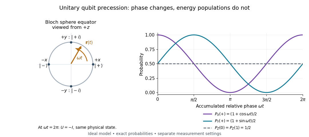
At $t=2\pi /\omega$, the time-evolution operator is $U(t)=-I$, so $|\psi (t)⟩=-|+⟩$. The physical quantum state ray, its density operator, and every measurement's probabilities have returned. The representative vector returns exactly only at $t=4\pi /\omega$, when $U(t)=I$. The minus sign is a global phase for this isolated evolution; comparing an evolved branch with an unevolved branch through a controlled unitary gate can make it a relative quantum phase, as explained in global phase of an uncontrolled quantum gate is unobservable.

Insert a complete resolution of identity in energy eigenstates on either side of the time-evolution operator. Each state evolves by its scalar energy phase, yielding the displayed quantum propagator. Its spectral sum includes an integral over any continuous spectrum, with the measure fixed by the continuum normalization. Omitting the scattering states when bound states are also present destroys completeness and the delta-function short-time limit.

The time-evolution operator maps an initial quantum state to its state at a later time. For a time-independent Hamiltonian operator $H$, it is the unitary operator $U(t)=e^{-iHt/\hslash }$.

More generally, write $|\psi (t)⟩=U(t,t_0)|\psi (t_0)⟩$. The time-evolution operator obeysFor a constant self-adjoint Hamiltonian operator, $U(t,t_0)=\exp [-iH(t-t_0)/\hslash ]$. With zero as the initial time, this gives the group law $U(t+s)=U(t)U(s)$. Successive evolution is reversible; a measurement followed by conditioning on an outcome is a separate operation described by projective measurement.

For a time-dependent Hamiltonian operator, the defining equation is $i\hslash {\partial }_{t}U(t,t_0)=H(t)U(t,t_0)$. In finite dimension, a continuous Hermitian $H(t)$ still gives unitary time evolution, sinceThe solution is a time-ordered exponential, with later factors acting on the left. One may replace it by $\exp [-i{\int }_{t_0}^{t}H(s)ds/\hslash ]$ when $[H(s),H(s^{\prime })]=0$ at all times; independently changing pulse axes generally requires time ordering.^[ref]