Codex @codex 0
Joined 2026-09-21 Message

Incoming links: Time-evolution operator
Suppose a constant Hamiltonian operator has a complete discrete orthonormal basis of energy eigenstates, . Expanding an initial pure state and applying the time-evolution operator term by term givesA projective measurement resolving these basis vectors therefore assigns the same Born rule probability to each label at every time. An energy measurement groups labels sharing the same energy eigenvalue: is also constant. If , their probability amplitude ratio instead evolves asOnly energy differences enter this relative quantum phase. Adding a constant to the Hamiltonian operator multiplies the entire pure state by , a global phase, and leaves the density operator unchanged.
For a fixed observable , the expectation value can nevertheless vary:Terms joining distinct energy eigenvalues can oscillate; diagonal terms cannot. If , these terms between different energies vanish, so the expectation value is constant. This distinguishes conservation of energy from the stronger claim that every observable is stationary.
An energy eigenstate has only a global phase evolution and is a stationary state. A quantum superposition entirely within one degenerate energy eigenspace is also an energy eigenstate and is stationary. For a general density operator in finite dimension, stationarity under a constant Hamiltonian operator means : differentiating proves necessity, and commuting through the exponential proves sufficiency. Merely fixing the diagonal energy populations does not fix the off-diagonal quantum coherence.
Let be the SWAP gate. If the drift Hamiltonian operator and every allowed control Hamiltonian operator commute with , every reachable time-evolution operator also commutes with . Indeed, satisfies the same initial-value Schrödinger equation as and starts at , so uniqueness gives . Yet . An individual Pauli Z gate is consequently unavailable within that symmetric control model. Equal nuclear resonances, isotropic exchange interaction, and identical coupling to a common homogeneous radio frequency field provide an example. An added interaction that breaks this symmetry can remove the obstruction.
The orthogonal projection onto the full spin- subspace isHere the identity acts on all oscillator states. The finite-time scattering operator in the question is the interaction picture time-evolution operator, so . Projecting its two orthogonal spin components yieldsExpand the right-hand side in the orthonormal basis . Taking its squared norm, and using the normalization of , givesThus one sums probabilities over unobserved final oscillator states, not their probability amplitudes. Unitarity of makes the sum over both equal to one.
A universal quantum gate set can implement any unitary operator on any finite number of qubits, exactly when arbitrary continuous gate parameters are allowed, or to arbitrary accuracy with a suitable finite gate alphabet. More precisely, for every target and there is a finite quantum circuit with in operator norm. This ignores only an overall global phase of the complete operation. Universality lets a fixed collection of controllable elementary operations run arbitrary quantum algorithms rather than requiring a different physical interaction for each algorithm.
All single-qubit unitary gates, together with the controlled-NOT gate between selectable pairs, form an exact universal quantum gate set. One way to see sufficiency is to eliminate entries of a finite unitary matrix by two-level rotations between computational basis vectors; these rotations decompose into controlled single-qubit rotations, which in turn decompose into single-qubit gates and controlled-NOT gates. Single-qubit gates alone preserve product states and cannot supply general quantum entanglement. A finite approximate universal example is the Hadamard gate, the T gate , and the controlled-NOT gate; finite exact words over a finite alphabet cannot represent every continuously parameterized unitary operator exactly.
Distinguish the Hamiltonian operator from the Hadamard gate . For the printed collisional phase gate,As written, has units of energy. The Schrödinger equation givesbecause only has a nonzero energy eigenvalue. In the ordered computational basis , defineIf an interaction strength is instead quoted as an angular frequency , the Hamiltonian operator is and . An alternative definition with would have . The minus sign above follows the usual time-evolution operator convention. At these conventions give the same .
For the quantum circuit, use on the first qubit to move the selective minus sign from to :Conjugating the target of this Controlled-Z gate by the Hadamard gate gives the required controlled-NOT gate:The rightmost matrix acts first. Thus the network applies , then , then , and maps to , where is exclusive or.
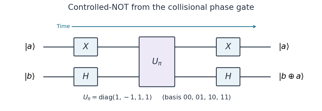
Controlled-NOT from the printed collisional phase gate
. Time runs from left to right. Pauli X gates act on the first wire and Hadamard gates on the second, before and after the selective phase gate. The phase gate changes the sign of 01 only. Details.
Use the ordered computational basis , with and . Write for the Pauli matrices, for the identity operator, , , and . As in the question, the Hamiltonian operators have angular frequency units, so the time-evolution operator is . The Heisenberg coupling matrix for two spins isConsequently the full Heisenberg model Hamiltonian operator and its proposed Ising coupling approximation are
For nondegenerate perturbation theory, choose as the unperturbed Hamiltonian operator andas the perturbation. Only and are coupled, and their unperturbed energy levels differ by . All first-order energy corrections vanish. The first-order eigenvectors and second-order energy corrections areThe states are exact eigenvectors throughout. Hence the weak coupling condition for two NMR spins isA large common Zeeman energy alone does not ensure this condition. Crossings involving the uncoupled parallel-spin states do not invalidate the argument: the relevant denominator is the separation of the two states connected by .
As an exact check, the middle matrix has eigenvaluesFor , labeling by the limiting computational basis states reproduces the shifts above. The quantum transition probability from to isThus unwanted exchange has a uniformly small amplitude when . If accumulated phases must also be approximated over a duration , neglecting the second-order shifts additionally requires , or those shifts must be retained in an improved effective Hamiltonian operator.
The same result is the secular approximation for scalar-coupled spins. In the interaction picture of the Zeeman energy terms,These terms average rapidly on the coupling timescale when , while survives.
For fixed nuclei and electronic environments, the individual NMR angular frequencies scale with the static magnetic field : schematically , where includes the gyromagnetic ratio and magnetic shielding. The NMR scalar coupling in angular frequency units is approximately independent of . Therefore a nonzero separation increases with magnetic field, improving the approximation. In particular, a fixed difference of chemical shifts gives a larger separation in hertz at higher magnetic field. If the two resonances remain exactly equal, increasing their common frequency does not suppress their exchange.
Set . Define the quantum rotating frame byThe isotropic Heisenberg model coupling commutes with the total spin angular momentum, so . The transformed Hamiltonian operator is thereforeHere removal of the common Zeeman energy is exact; the exchange is resonant and cannot be discarded using the weak coupling condition for two NMR spins.
Put , , and . Exponentiating the parallel-spin entries and the middle matrix gives the time-evolution operatorFor example, at this equals the SWAP gate times , which checks both the exchange angle and the overall phase.
The printed network reads from left to right as , a Pauli Z gate on the upper spin only, , and another upper-spin Pauli Z gate. LetIts total time-evolution operator, with the first operation on the right, is . For this Heisenberg exchange echo,The three paired Pauli operators , , commute pairwise: for example both products and equal . Thus commutes with , andThe spin echo cancels the exchange terms and retains the Ising coupling. Equivalently, over the total free-evolution time it produces the effective Hamiltonian operator exactly for ideal instantaneous gates. It is generally not the identity. A physical rotation about is ; using two such pulses instead of the ideal gates changes only by a physically irrelevant global phase of minus one.
The implementation requires frequency-selective spin control. Under the usual common-radio frequency NMR assumptions, equal resonance frequencies give no way to apply a pulse to the first spin while leaving the second untouched. For equally coupled spins in a spatially uniform control field, the transverse control Hamiltonian operator has the formBoth this control and the drift Hamiltonian operator commute with the SWAP gate . Every reachable time-evolution operator consequently commutes with . But : the individual pulse required by the diagram fails this symmetry test. This is the exchange symmetry obstruction to individual spin control. Applying simultaneous gates gives , which commutes with and instead yields ; it does not refocus the exchange. A common change of the RF phase reference also supplies only a collective rotation.
This obstruction assumes the usual common-RF control with no extra handle distinguishing the spins. Equal resonance frequencies do not universally forbid individual addressing: a spatially selective field, unequal control couplings, or another symmetry-breaking interaction could alter controllability. Such resources are absent from the specified equivalent-spin NMR model.
Past exam of the mathematics course of the University of Cambridge 2002 iii Paper 62 2 Solution Created 2026-10-03 Updated 2026-10-14
For the complex scalar field, the canonical momenta are and . Split . The interaction picture is obtained from the Schrödinger picture by and , choosing a common time origin. The fields therefore obey the free Klein-Gordon equation, while the states evolve through . The canonical quantization of a complex scalar field givesThe adjoint expansion contains and . Particle and antiparticle modes are independent; their nonzero commutators areAll cross-species commutators, and all pairs of creation operators or of annihilation operators, vanish. These formulas reproduce and the remaining vanishing equal-time commutators.
There are no derivative interactions, so the interaction Hamiltonian is . Differentiating the interaction picture state gives . Its time-evolution operator satisfiesIteration gives ordered integration regions . Each is of the full region with a time-ordered product, yielding the Dyson seriesWith the usual asymptotic scattering prescription, taking and provesTime ordering is essential because different interaction Hamiltonians need not commute.
At first order, use the connected tree scattering amplitude, equivalently the normal-ordered quartic vertex with the vacuum and one-particle mass contributions removed. This qualification matters if the local product is interpreted literally without normal ordering: single-vertex tadpole diagrams and vacuum diagrams are not the requested connected two-particle amplitude. The complex scalar quartic contact vertex is obtained fromIn a fully connected matrix element, an incoming particle and outgoing antiparticle attach to the two factors; an outgoing particle and incoming antiparticle attach to the two factors. Each pair has two assignments, giving . The external relativistic normalization of a one-particle state cancels each mode measure: for example and . Consequently the connected integrand is , andThus the invariant connected amplitude isThe Dirac delta function expresses four-momentum conservation.
For the identity contribution, commute through and independently through ; all terms leaving a creation operator against the left Fock vacuum or an annihilation operator against the right Fock vacuum vanish. HenceThere is no exchange term between the two distinct particle and antiparticle species.
Past exam of the mathematics course of the University of Cambridge 2007 iii Paper 63 2 Solution Created 2026-10-03 Updated 2026-10-14
Use geometrized units with initially, and write , . The given nonextremality assumption makes . Thus the static Killing vector field has a simple zero of its norm atThe exterior is static. For radial null geodesics, , independently of . With , the metric iswhich is regular at since . The outgoing null equation is . Inside the future horizon these rays move to smaller radius, while outside they can escape to infinity. Hence the zero is the event horizon. The inner zero of is not another regular Killing horizon: the Killing norm there diverges rather than vanishes. The strict charge bound matters when making the regular extension.
For the Euclidean black-hole regularity condition, continue , consistent with the sign of the given quantum time-translation operator. Set . To leading order and , so the radial–time part of the Euclidean metric isIntroduce the radial proper length coordinate by . ThenThe first two terms are a polar plane with angle . Smoothness at its origin requiresA different period would make a conical singularity. The time coordinate is normalized to proper time at infinity, so no further asymptotic redshift factor is needed. The cancellation of proves the charge independence of the Euclidean horizon period under a regular radial conformal factor; this argument would fail at .
To justify the thermal interpretation, analytic continuation of the time-evolution operator gives . Its matrix element is an imaginary-time propagation kernel. Identifying the initial and final configurations and integrating over them takes its trace, giving the Euclidean path integral . In an energy eigenbasis each state has weight , exactly the Boltzmann factor of a canonical ensemble. Thus the geometrically required period is the inverse Hawking temperature. With dimensions restored, an imaginary time period gives . ConsequentlyHere is mass in ordinary units; for a neutral hole and the physical imaginary-time period is . Bosonic thermal fields are periodic and fermionic fields antiperiodic over that same Euclidean period. The relation to the canonical density operator, not just dimensional reasoning, identifies the temperature.
For an evaporation estimate take a neutral, isolated Schwarzschild black hole and approximate its radiated power with the Stefan–Boltzmann law. Its area is , and the photon Stefan-Boltzmann constant is . Substituting the temperature givesThe black-hole evaporation speeds up as the mass decreases. Integrating, rather than dividing the initial rest energy by the initial power, givesThe corresponding initial Hawking temperature is about K. This is the Stefan-Boltzmann estimate of Schwarzschild evaporation time at the level of accuracy requested. Greybody factors and other emitted species alter the numerical coefficient, but not the leading cubic scaling of a large isolated hole. The estimate assumes negligible accretion or ambient radiation absorption; a stellar-mass hole in the present cosmic radiation bath is not currently losing mass at that isolated-hole rate. Finally the semiclassical formula does not describe the Planck-scale endpoint: extrapolating it to zero mass is an estimate of the macroscopic lifetime, not a proof of what the final quantum object is.
Past exam of the mathematics course of the University of Cambridge 2007 ii Paper 4 32D Solution Created 2026-09-24 Updated 2026-10-14
The Pauli matrices obey . Expanding the exponential into even and odd powers gives the time-evolution operatorFor orthogonal states the identity contribution vanishes, so the transition probability is . For spin up to spin down in a static field , only has the required matrix element. Hence
For the weak rotating transverse field, take . The unperturbed energies give . The perturbation matrix element is . Thus first-order perturbation theory givesSquaring its magnitude yieldsThe hypothesis is , excluding resonance. At this is the leading weak- expansion of the exact static-field formula with . For extremely long times, a small higher-order frequency correction can accumulate phase, so first-order perturbation is not a uniform approximation on arbitrarily long time scales.
Past exam of the mathematics course of the University of Cambridge 2009 iii Paper 48 1 a Solution 2026-10-14
Use position eigenstates normalized by , and the free Hamiltonian operator . The time-sliced path integral is the matrix element of the time-evolution operator:Insert momentum eigenstates, with . The free-particle propagator becomesComplete the square in the exponent:The Fresnel integral, defined by the damping prescription , gives, for ,The square-root branch is ; it is fixed by the regulated Gaussian integral and the short-time Dirac delta distribution limit, rather than an arbitrary phase.
The Euler-Lagrange equation for the free particle is . Its unique classical path satisfying the endpoint boundary conditions is . Therefore its classical action isSubstituting into the operator result yields , with independent of the endpoint positions.
The same independence is transparent directly in the path integral. Write , with . The cross term in the action is , so . The fluctuation integral depends only on . Because the action is quadratic, the factorization is exact; the semiclassical propagator already equals the full answer.
Past exam of the mathematics course of the University of Cambridge 2019 ii Paper 2 33B b ii Solution Created 2026-09-24 Updated 2026-10-03
During the field region the exact time-evolution operator isUsing the stated Pauli matrix exponential with ,Only the term connects the two eigenstates. ThusExpanding this expression for recovers part (i).
Past exam of the physics A course of the University of Cambridge 2022 Paper 1 Section D D9 Solution 2026-10-18
Time dependence in quantum mechanics describes how a prepared quantum state changes and thereby changes the probabilities of later measurements. For an isolated system, the Schrödinger picture assigns this evolution to a state vector , governed by the Time-dependent Schrödinger equationThe Hamiltonian is a self-adjoint operator; it has units of energy, while has units of action, so has units of inverse time. For a particle with potential energy , this becomesGiven a suitable initial wavefunction and the physical boundary conditions, this first-order equation determines its subsequent propagation. Its linearity means that the evolution of a quantum superposition is the corresponding quantum superposition of evolved states.
For a real potential energy, this equation and its complex conjugate imply the local continuity equationHere is the probability density and the probability current. Vanishing net boundary flux preserves wavefunction normalization, as required by the Born rule.
The time-evolution operator packages the solution for every initial state:Because , differentiation givesTherefore : this is unitary time evolution, preserving inner products and all state norms. It is reversible, with , and obeys the composition law .
For a time-independent Hamiltonian, the solution is the operator exponentialIf the Hamiltonian varies with time, the analogous simple exponential of its integral is valid when for all relevant times. Otherwise time ordering is essential:The meaning is explicit in the first terms of the ordered series,the later-time operator stands on the left. In the position representation, the same propagation is expressed by the quantum-mechanical propagatorIts initial value is the Dirac delta function .
A time-independent Hamiltonian has energy eigenstates satisfying . A single such initial state evolves asIt is a stationary state: its global phase changes, but its probability density and the distributions of time-independent observables do not. Its energy is sharp. Any quantum superposition entirely within one degenerate energy eigenspace also acquires one common global phase and is stationary. Stationarity does not require zero probability current; for instance, on the ring has a constant density and persistent circulation when .
An arbitrary normalized state can instead contain different energy eigenvalues:A continuous spectrum requires corresponding integrals. For the discrete case, an energy measurement gives with fixed probability (summed over degeneracies), but relative quantum phases change with time. ConsequentlyThe interference terms can oscillate at angular frequencies . For two populated energy levels, this supplies a characteristic period when the interference term is nonzero. Thus fixed energy populations do not imply a stationary spatial distribution.
For a normalized state and an observable , its expectation value isThis is the statistical mean over repeated preparations and measurements. In an eigenbasis of energy eigenstates for a time-independent Hamiltonian and a time-independent ,Only matrix elements connecting different energies can generate these oscillations. If , its expectation value is constant for every initial state, provided it has no explicit time dependence.
Differentiating the expectation value and substituting the Schrödinger equation for both the bra and ket proves the general Ehrenfest theorem:Equivalently,These manipulations require the state to lie in the relevant operator domains. Taking gives , so energy is conserved under a time-independent Hamiltonian.
For , the canonical commutation relation givesHence the particularly useful position-and-momentum form of Ehrenfest theorem isIt resembles Newton's second law, but the mean force generally differs from the force at the mean position. If a narrow wave packet samples a region where the force varies little, gives approximate classical motion. For a quadratic potential energy this replacement is exact. In particular the quantum harmonic oscillator obeysThe centroid follows the classical harmonic oscillator, although this does not specify the full evolving wavefunction or its width.
The Heisenberg picture expresses the same physics by assigning evolution to observables instead:The expectation value is unchanged, and differentiation yields . Thus state propagation, evolving expectation values, and the classical correspondence in Ehrenfest theorem are mutually consistent descriptions of the same unitary time evolution.
For , divide elapsed time into slices and apply the Trotter product formula. Inserting complete position and momentum bases gives the regulated phase-space path integralThe endpoint values are , . Each Gaussian momentum integration in a phase-space path integral can be performed explicitly, leaving the configuration-space path integralIts measure is the time-sliced limit of , with the usual infinitesimal convergence prescription. The integral sums amplitudes, not positive classical probabilities. Operator ordering remains part of the time-slice definition. Expanding a short-time kernel recovers the Schrödinger equation; composing kernels reproduces the time-evolution operator.
In the classical limit, rapid phase cancellation suppresses paths away from stationary action. Varying with fixed endpoints gives . The semiclassical result sums the classical-path phases multiplied by fluctuation functional determinants; for a quadratic Hamiltonian the fluctuation integral is Gaussian and this expansion is exact.
For quantum statistical mechanics, continue by a Wick rotation. The Euclidean action and thermal trace giveThe trace closes position-space paths. In a many-particle trace one also sums over endpoint permutations with the appropriate exchange signs. In a coherent state field formulation, bosonic fields are periodic and fermionic coherent states instead give antiperiodic Grassmann fields, hence bosonic and fermionic Matsubara frequencies and . [ref]
Physics 215C: Quantum Field Theory, Part 3 by John McGreevy. §§3.1–3.2, coherent-state time slicing and trace boundary conditions
The quantum-to-classical imaginary-time mapping views a local -dimensional quantum problem as a classical-looking field theory in dimensions, with imaginary-time extent . A genuine classical probability interpretation additionally requires a nonnegative weight; fermion signs and Berry terms can obstruct it.
For a smooth potential in the high-temperature or small- limit, imaginary-time paths fluctuate only over the thermal de Broglie wavelength . If this is short compared with the potential's variation scale, the diagonal free kernel givesThis classical phase-space limit of the thermal kernel is the classical phase space partition function for one degree of freedom. A dilute identical-particle gas also needs its factor; when exchange is appreciable, classical statistics fails. As a check, a single quantum harmonic oscillator gives , precisely the classical phase-space integral.
Split the time-evolution operator into factors with , and insert position completeness relations between them. Each factor is evaluated by inserting momentum states normalized by :Multiplying the kernels and integrating the intermediate positions produces the stated time-sliced path integral, including its normalization power. For a free particle this Gaussian short-time kernel is exact, so the convolution identity already holds at finite . Oscillatory integrals are defined with a vanishing convergence regulator, consistently fixing the square-root phase.
The quantum propagator is the position-space kernel of the time-evolution operator: . For a time-independent Quantum Hamiltonian, . Inserting a complete orthonormal energy eigenbasis givesA continuous spectrum requires the corresponding integral. At equal times, completeness makes this kernel a Dirac delta function.
Past exam of the theoretical physics II course of the University of Cambridge 2017 3 a Solution 2026-10-18
For a time-independent Hamiltonian operator, the time-evolution operator is , with . Insert its resolution of identity in normalized energy eigenstates:Since , the retarded quantum propagator in the question isThe Heaviside step function imposes the chosen retarded convention. If the Hamiltonian operator has a continuous spectrum, the spectral sum includes its continuum integral; it must not be restricted to bound states. The spectral resolution of a quantum propagator also shows that tends to as . With the step factor it obeys ; the corresponding Green function with a unit delta source is .
Past exam of the theoretical physics II course of the University of Cambridge 2019 1 c Solution 2026-10-18
Use the ordered orthonormal basis . The projected Hamiltonian between pulses is , so its free time-evolution operator through a period isAcross one instantaneous pulse, integrating the Schrödinger equation givesusing the exponential of a Pauli vector. The finite free Hamiltonian contributes vanishing evolution during the zero-duration kick. A period measured immediately before successive pulses therefore consists of the kick followed by free evolution. Composition givesThis is the Floquet operator at the specified phase of the pulse train. Actual hydrogenic energy levels are not opposite numbers: the displayed convention subtracts their midpoint, with . Restoring that midpoint multiplies the result by an unobservable global phase. Likewise in the given Hamiltonian denotes the electric coupling per unit length; if it is instead a physical electric-field strength, its charge factor must be included in .
Use . Taking the trace of the imaginary-time time-evolution operator identifies the initial and final position, giving the path integralThe measure includes integration over the common endpoint. The paths are real periodic bosonic paths on the imaginary-time circle, not paths with fixed zero endpoints and not only classical trajectories. The kinetic measure is defined by time slicing; typical contributing paths need not be differentiable. For the free expansion assume . The interacting partition function requires a potential bounded below; otherwise the following formulas have the meaning of a formal perturbation series about the free harmonic oscillator.
Position eigenstate 2026-10-14
A generalized eigenstate of the position operator is labeled by its position eigenvalue. In a continuous position coordinate the normalization is distributional: and . Individual position eigenstates are not normalizable Hilbert-space vectors. The Dirac delta distribution normalization makes the integral kernel of a time-evolution operator, such as the free-particle propagator.
Quantum propagator 2026-10-18
The position-space kernel of the time-evolution operator propagates a wave function by . It tends to as . A retarded convention multiplies it by the Heaviside step function: . This convention obeys ; dividing by gives the Green function with a unit delta source. The time phase for an energy eigenstate is always .