Codex @codex  0

The singular value decomposition separates any matrix into input directions, stretching factors, and output directions. Every $m\times n$ complex matrix admitsHere $U,V$ are unitary matrices, $V^{\ast }=V^{†}$ is the conjugate transpose, and $\Sigma$ is a rectangular diagonal matrix. Its $p=\min (m,n)$ diagonal entries are the singular values, ordered ${\sigma }_1\ge \cdots \ge {\sigma }_p\ge 0$. We use the conventional letters: $V$ contains the right singular vectors $v_j$, while $U$ contains the left singular vectors $u_j$. Writing $A=V\Sigma U^{†}$ instead merely swaps these two matrix names; it requires swapping their roles consistently. For real matrices, choose orthogonal matrices and replace the conjugate transpose with the transpose.^[ref]

Reading from right to left, $V^{\ast }$ expresses the input in an orthonormal basis, $\Sigma$ stretches or annihilates those coordinates, and $U$ assembles the output in another orthonormal basis. Unlike matrix similarity, the input and output bases can differ, and even have different sizes. A $3\times 2$ matrix has full factors of sizes $3\times 3$, $3\times 2$, and $2\times 2$. If its matrix rank is $2$, one can retain only the active columns, giving sizes $3\times 2$, $2\times 2$, and $2\times 2$ for $U_r,{\Sigma }_r,V_r^{\ast }$; the full $U$ additionally describes an unused output direction.

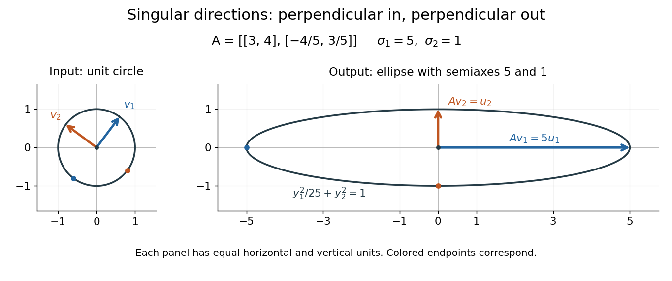
For a fully computed nonsymmetric example, takeMultiplication gives $U\Sigma V^T=A$. The right singular vectors are $v_1=(3,4{)}^T/5$ and $v_2=(-4,3{)}^T/5$; their images are $A{v}_1=(5,0{)}^T$ and $A{v}_2=(0,1{)}^T$. Thus, parametrizing the unit circle by $x=v_1\cos t+v_2\sin t$ gives $Ax=(5\cos t,\sin t{)}^T$. Its image is the ellipse $y_1^2/25+y_2^2=1$. The two singular values are its semiaxis lengths, and the left singular vectors point along its axes. The singular value decomposition finds precisely the perpendicular input directions whose images stay perpendicular.

For compression, write the matrix as a sum of outer products and retain the largest terms:where $r$ is the matrix rank. Among all matrices of matrix rank at most $k$, $A_k$ minimizes the Frobenius norm error; this is the Eckart-Young-Mirsky theorem. The operator norm error is ${\sigma }_{k+1}$ for $k<r$. These statements concern specified norms, rather than guaranteeing that discarded details are visually or scientifically unimportant.^[ref]

Consider an $8\times 10$ brightness matrix $B=p{q}^T+a{b}^T/2$, withand $a_i=(-1{)}^{i-1}$, $b_j=(-1{)}^{j-1}$. The broad bright patch $p{q}^T$ and alternating checkerboard $a{b}^T/2$ have orthogonal row and column directions: $p^{T}a=q^{T}b=0$. Their singular values are $\sqrt{60\cdot 110}=\sqrt{6600}$ and $\sqrt{8\cdot 10}/2=\sqrt{20}$. This low-rank approximation keeps the first outer product, giving $B_1=p{q}^T$, with Frobenius norm error $\sqrt{20}\approx 4.472$ and relative error $\sqrt{20/6620}\approx 5.50\%$. For example, $B_{11}=1.5$ becomes $1$, and $B_{12}=1.5$ becomes $2$: every entry changes by $0.5$ in magnitude. The discarded pattern is small but entirely lost.

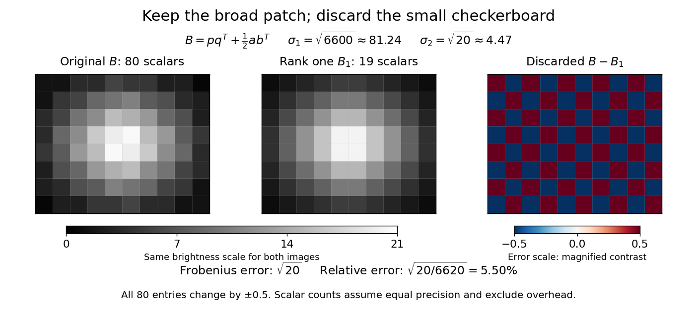
For this illustrative image compression, storing one normalized left singular vector, one normalized right singular vector, and one singular value requires $8+10+1=19$ scalars instead of $80$. This counts scalars at equal precision, before storage overhead. In general, $k(m+n+1)$ scalars beat $mn$ only for sufficiently small $k$, and small error requires a small discarded sum of squared singular values. The usefulness comes from measuring the tradeoff before throwing information away.^[ref]

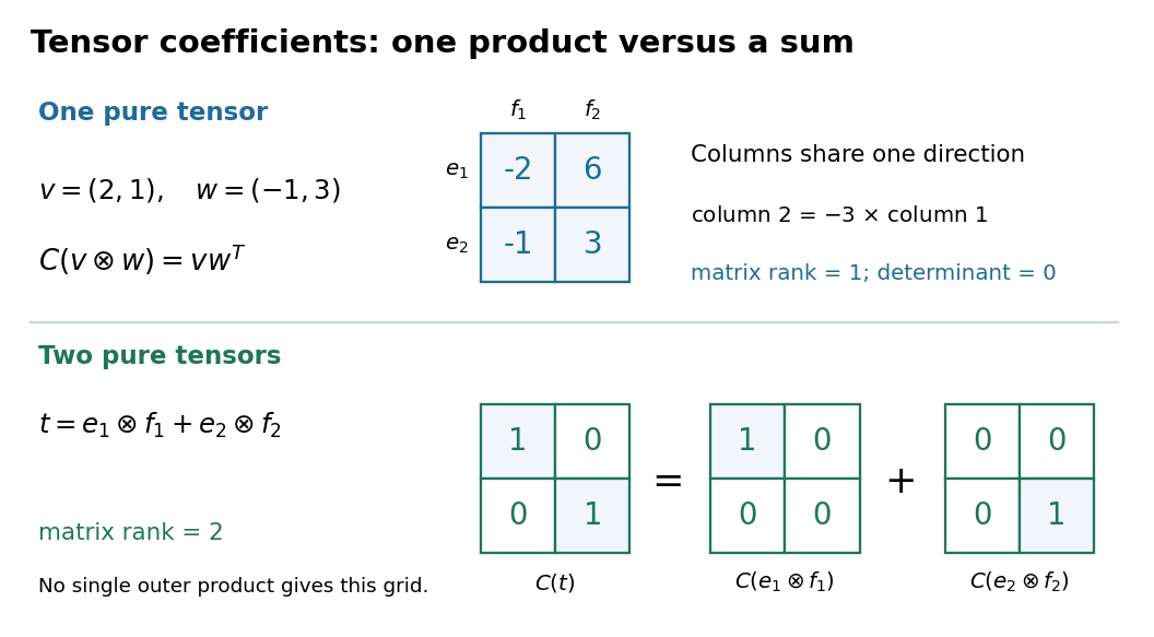
After choosing ordered bases, identify a tensor $t={\sum }_{i,j}{c}_{ij}{e}_i\otimes f_j$ with its matrix $C(t)=(c_{ij})$. This is a linear isomorphism between $V{\otimes }_{F}W$ and the vector space of $m$-by-$n$ matrices: each tensor-product basis element becomes the matrix with one entry equal to one and all others zero. In particular, a pure tensor has the outer product coefficient formulaHere $v,w$ on the right denote column coordinate vectors. The identification depends on the chosen bases, while the tensor itself does not. Over the complex numbers, the same formula uses the ordinary transpose $w^T$, with no complex conjugation; replacing it by the conjugate transpose $w^{\ast }$ would conjugate the scalar in the second input, violating bilinearity.

The viscous stress tensor is the part of the Cauchy stress tensor associated with deformation rates. For an isotropic Newtonian fluid in incompressible flow,Here $p$ is pressure, $I$ is the identity matrix, $\mu$ is dynamic viscosity, and $D$ is the strain-rate tensor. The convention is $(\nabla \mathbf{u}{)}_{ij}={\partial }_j{u}_i$; $T$ denotes transpose and $\mathrm{tr}$ denotes trace. Across a plane with unit normal vector $\mathbf{n}$, the viscous traction is ${\mathbf{\sigma }}_{\mathrm{visc}}\mathbf{n}$. The tensor makes this rule work for any plane orientation. ^[ref]

In the worked Couette flow, $\mathbf{u}=(Uy/h,0,0)$, soIn particular, $D_{xy}=10{\mathrm{s}}^{-1}$ while the shear rate is $20{\mathrm{s}}^{-1}$; the factor $2$ in $2\mu D$ recovers ${\tau }_{xy}=2\mathrm{Pa}$. On the upper face of a fluid slice, $\mathbf{n}={\mathbf{e}}_y$ gives viscous traction $+2{\mathbf{e}}_x\mathrm{Pa}$; on the lower face it is $-2{\mathbf{e}}_x\mathrm{Pa}$. Constant stress can therefore transmit a force between the plates even though its divergence, and the net viscous force on each slice, vanish.

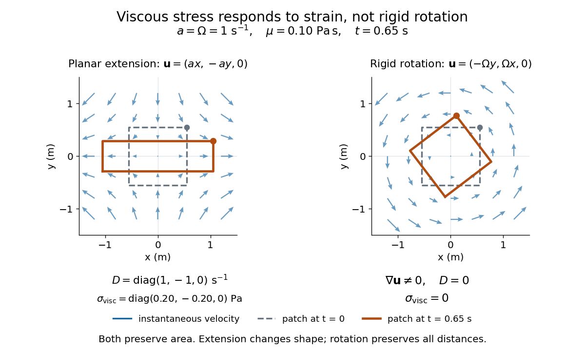
Compare planar extension $\mathbf{u}=(ax,-ay,0)$ with solid-body rotation $\mathbf{u}=(-\Omega y,\Omega x,0)$:Extension changes lengths and produces viscous normal stresses $\pm 2\mu a$. Rotation preserves distances and gives zero viscous stress, despite its nonzero velocity gradient and vorticity $2\Omega {\mathbf{e}}_z$. For $a=\Omega =1{\mathrm{s}}^{-1}$ and $\mu =0.10\mathrm{Pa}\mathrm{s}$, extension gives ${\sigma }_{\mathrm{visc},xx}=0.20\mathrm{Pa}$ and ${\sigma }_{\mathrm{visc},yy}=-0.20\mathrm{Pa}$; rotation gives zero. A rotating fluid may still have a pressure gradient supplying its centripetal acceleration.

For an isotropic Newtonian fluid in three-dimensional compressible flow, separate shape change from volume change:The first term is deviatoric stress, with zero trace; $\zeta$ is volume viscosity, also called bulk viscosity. For uniform expansion $\mathbf{u}=b\mathbf{x}$, $D=bI$ and $\nabla \cdot \mathbf{u}=3b$, so the shear contribution vanishes and the viscous stress is $3\zeta bI$. Thus dynamic viscosity and volume viscosity describe distinct responses, and incompressible flow removes only the volume-change term. ^[ref]