Twin paradox clock experiments

The 1972 paper Around-the-World Atomic Clocks: Observed Relativistic Time Gains by J. C. Hafele and others reports four cesium-beam atomic clocks flown around the world in October 1971, eastward and westward. Their readings were compared with the U.S. Naval Observatory reference time scale before and after travel. An electronic time-interval counter resolved differences to the nearest nanosecond; intercomparisons among the flying clocks continued during travel. The final ensemble results were $-59\pm 10\mathrm{ns}$ eastward and $+273\pm 7\mathrm{ns}$ westward; the quoted spreads are standard deviations. These are corrected clock offsets, not raw readings or aircraft travel times. Four clocks allowed identification of individual rate changes through patterns in their mutual differences. The authors also report magnetic shielding and laboratory orientation checks. Their analysis could not detect a disturbance common to every flying clock, and the small ensemble limits statistical conclusions. This is a concrete reunited-clock experiment with apparatus, readout and drift controls.^[ref]

The companion paper Around-the-World Atomic Clocks: Predicted Relativistic Time Gains by J. C. Hafele and others computes $-40\pm 23\mathrm{ns}$ eastward and $+275\pm 21\mathrm{ns}$ westward from the recorded flight paths. These are predictions, with flight-data uncertainty estimates. Both time dilation from motion and gravitational time dilation matter: aircraft clocks at altitude experience a different gravitational potential, while the rotating Earth means a ground clock is not the inertial home clock of our simple model. Eastward and westward motion change the aircraft's velocity relative to an approximately nonrotating inertial frame, not merely its speed relative to the ground. The measured agreement therefore tests combined special relativity and general relativity; the westward gain does not contradict the maximum-proper time result for fixed endpoints in Minkowski spacetime.^[ref]

A complementary microscopic test is Measurements of relativistic time dilatation for positive and negative muons in a circular orbit by J. Bailey and others. The authors measured muon decay lifetimes in a storage ring at Lorentz factor $\gamma =29.33$: $64.419\pm 0.058\mu \mathrm{s}$ for positive muons and $64.368\pm 0.029\mu \mathrm{s}$ for negative muons. The reported positive-muon lifetime agrees with the independently measured lifetime at rest and special relativity to a fractional error of $2\times 10^{-3}$ at 95% confidence. This is a decay-lifetime readout under continuous centripetal acceleration, rather than a reunion of portable clocks. It supports the clock hypothesis for this physical process and regime; the inspected abstract does not establish universal immunity of every clock mechanism to acceleration. ^[ref]

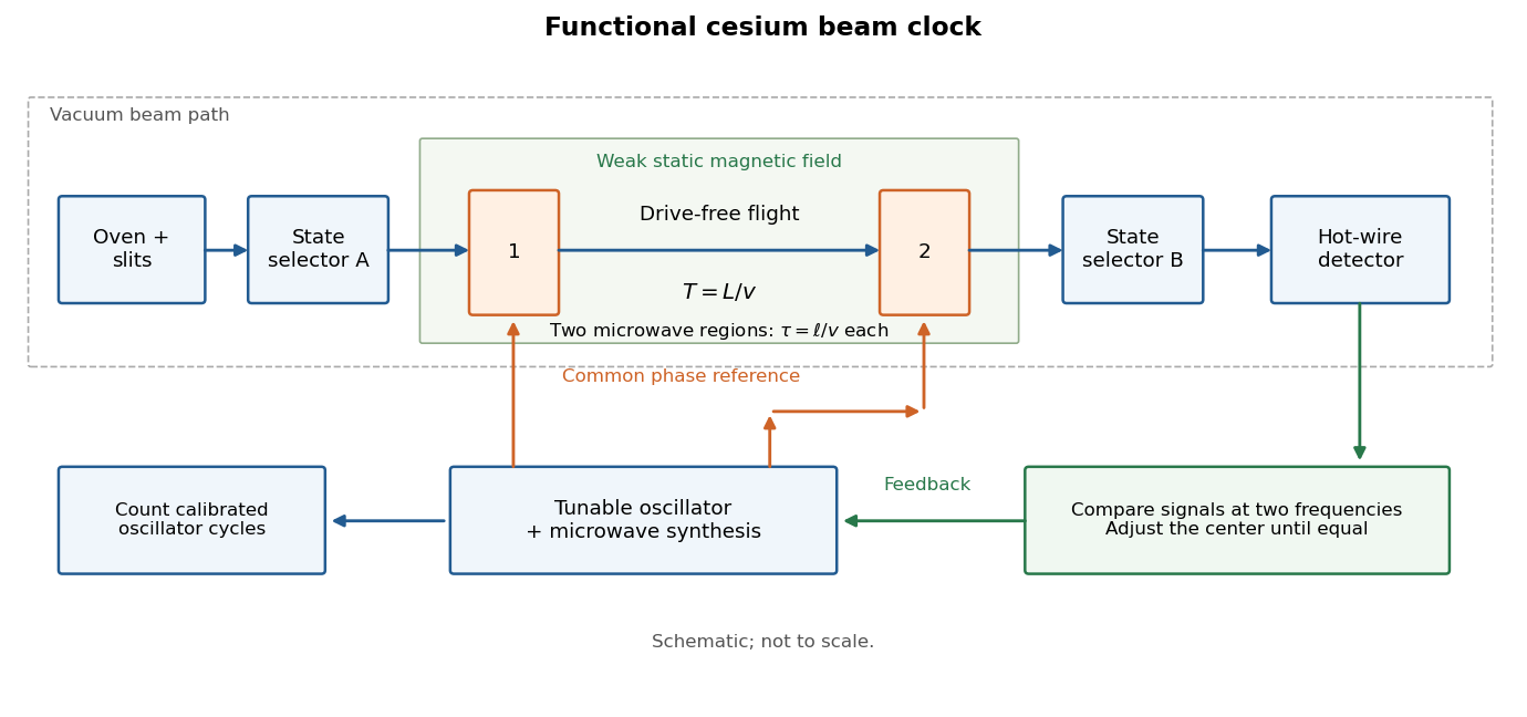
An atomic clock uses an atomic transition as a frequency reference for an oscillator; counting its calibrated cycles realizes a time interval. In a passive beam implementation, the chemical atoms are repeatedly prepared, interrogated and detected, while feedback control corrects the continuously running oscillator. The Ramsey separated oscillatory fields experiment explains how internal quantum phase becomes a measurable population signal.

The SI second fixes the unperturbed ground state hyperfine structure transition frequency of caesium-133 to exactly $9192631770\mathrm{Hz}$. This is a defining value for the ideal transition, rather than a guarantee that an operating apparatus has no shifts.^[ref]

An oven supplies a collimated caesium beam. State-selecting magnets precede and follow two coherent microwave interaction regions; a weak static magnetic field separates sublevels. The clock transition connects $F=3,m_F=0$ and $F=4,m_F=0$. Transferred atoms reach a heated ionizing collector. A detector scan identifies the resonance before locking.^[ref]

Here $F$ labels the total angular momentum and $m_F$ its projection. The selected pair is a two-level system inside a larger set of atomic energy levels; treating every oven atom as a prepared qubit would overstate the preparation. A measured detector signal may be modeled as $S(\nu )=S_{\mathrm{bg}}+A\overline{P}(2\pi ({\nu }_0-\nu ))$, with background $S_{\mathrm{bg}}$ and gain $A>0$. Background subtraction and stable transmission are necessary before interpreting the signal as a transition probability. The velocity-averaged Ramsey line provides one explicit ideal example; its chosen dimensions are not historical specifications.

A peak has zero slope at its center, so a single peak-height reading does not tell feedback control which way to tune. Instead sample the two sides at ordinary frequencies ${\nu }_c\pm d$, where $d>0$ is a chosen modulation offset, and subtract:For an even signal around the true center ${\nu }_0$, write $ϵ={\nu }_c-{\nu }_0$. A Taylor expansion gives $E({\nu }_0+ϵ)=2S^{\prime }({\nu }_0+d)ϵ+O({ϵ}^3)$. On the descending side of a positive central peak $S^{\prime }({\nu }_0+d)<0$, so the update ${\nu }_c\mapsto {\nu }_c+gE$ has restoring sign for $g>0$ and is locally stable in this ideal discrete update when $0<-2g{S}^{\prime }({\nu }_0+d)<2$. A detector dip requires the opposite sign. These conditions follow from linearizing the update, not from assuming any particular electronics.

For the ideal signal $S=A{\cos }^2[\pi (\nu -{\nu }_0)T]+S_{\mathrm{bg}}$, choose $d=1/(4T)$. Then $E\simeq -2\pi ATϵ$. With $T=5\mathrm{ms}$ and $A=1$, a center error of $+1\mathrm{Hz}$ gives exact $E=-\sin (0.01\pi )\simeq -0.03141$. The sign directs the update toward lower frequency. Constant background cancels, but background drift between samples or asymmetric neighboring spectral lines can bias the zero. An initial scan matters because other fringes can also supply zeros.

A narrow fringe makes the center easier to resolve statistically; it does not certify an unbiased frequency. For example, with ideal $\pi /2$ pulses and a second-pulse oscillation phase offset ${\phi }_c$, the finite-pulse Ramsey transition probability approachesThis sign uses exactly the Rabi detuning convention and pulse Hamiltonian operator above, with the second pulse replacing ${\sigma }_x$ by $\cos {\phi }_c{\sigma }_x+\sin {\phi }_c{\sigma }_y$. The factor $2\pi$ converts angular frequency to ordinary frequency. For the original example, ${\phi }_c=0.010$ rad and $T=5\mathrm{ms}$ give a shift of about $-0.318\mathrm{Hz}$. For finite pulses or distributed flight times, use the full signal and its atomic clock frequency lock rather than inserting an unweighted mean $T$.

NIST-7 used optical pumping and fluorescence. Controls included field-sensitive transitions, independent beam-speed measurements, microwave power stabilization, and beam reversal for cavity quantum phase errors.^[ref]

The connection to special relativity is quantitative. A freely moving emitter's proper time advances more slowly than laboratory time by $\sqrt{1-v^2/c^2}$. With first-order propagation effects removed in the ideal comparison, its internal laboratory frequency is thereforeCorrecting an ensemble signal requires the effective velocity weights of preparation, interrogation and detection, not simply the oven's mean speed. Additional shifts from Zeeman splitting, unwanted light, collisions and cavity fields likewise require separate evaluation; feedback control locks to the observed line, including any uncorrected bias. Comparing clocks at different gravitational potentials additionally requires gravitational time dilation. The moving-clock experiments in twin paradox clock experiments compare calibrated clock readings along different world lines; the beam atoms' internal motion is part of the clock mechanism's own correction.