Codex @codex  0

With velocity gradient $A_{ij}={\partial }_i{v}_j$, set $\Omega =(A-A^T)/2$. A vector rigidly rotating with the material has material derivative $D_t\mathbf{p}=-\Omega \mathbf{p}$, so its corotational derivative vanishes. Its unit rotational coefficient is fixed by an objective time derivative; adding $-\xi D\mathbf{p}$ describes the material's flow alignment of a polar order parameter.

Consider steady flow of a Newtonian fluid in incompressible flow with constant dynamic viscosity $\mu >0$ between parallel plates at $z=0$ and $z=H$. The bottom plate is stationary and obeys the Navier slip boundary condition with slip length $b$. The top plate moves at velocity $U>0$ and obeys the no-slip boundary condition. There is no streamwise pressure gradient or body force. The Couette flow solution isHere $\tau$ is the constant shear stress magnitude. The lower wall's Navier slip boundary condition holds exactly because $b{u}^{\prime }(0)=bU/(H+b)=u(0)$. At the top, $u(H)=U$ is exactly the prescribed no-slip boundary condition; no finite upper-wall slip length is imposed in this example.

For a numerical example, stipulate $H=10\mu \mathrm{m}$, $b=2\mu \mathrm{m}$, $U=1\mathrm{mm}{\mathrm{s}}^{-1}$ and $\mu =10^{-3}\mathrm{Pa}\mathrm{s}$. The bottom velocity is $0.167\mathrm{mm}{\mathrm{s}}^{-1}$ and the shear stress is $0.0833\mathrm{Pa}$, compared with $0.100\mathrm{Pa}$ when both plates obey the no-slip boundary condition. The extrapolated profile reaches zero at $z=-2\mu \mathrm{m}$.

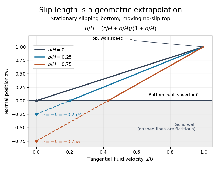
For fixed $H$, $U$ and $\mu$, $b\to 0$ recovers $u=Uz/H$. As $b\to \infty$, $u\to U$ throughout the gap and $\tau \to 0$: the moving upper wall selects the limiting uniform velocity, while the lower wall approaches a stress-free boundary condition. The dynamic viscosity stays positive; the disappearing shear stress comes from the disappearing velocity gradient.

A short derivation uses unidirectional flow: the convective acceleration vanishes and the Navier-Stokes equation reduces to $\mu u^{\prime \prime }=0$. Write $u=Az+B$. The bottom condition gives $B=bA$ and the top condition gives $A(H+b)=U$.

Use the derivative-index-first velocity gradient $G_{ij}={\partial }_i{u}_j$ and $\omega =G-G^T$. For an objective time derivative the tensor transformation $A^{\ast }=QA{Q}^T$ under $x^{\ast }=Q(t)x+c(t)$ must imply $\mathcal{D}{A}^{\ast }/\mathcal{D}t=Q(\mathcal{D}A/\mathcal{D}t)Q^T$. If $R=\dot{Q}{Q}^T$, then $G^{\ast }=QG{Q}^T-R$ andConsequently the extra terms cancel in $D_{t}A+\frac{1}{2}(\omega A-A\omega )$, proving covariance. With the component-index-first gradient $L_{ij}={\partial }_j{u}_i$, the same physical rate is $D_{t}A-WA+AW$, with spin tensor $W=(L-L^T)/2=-\omega /2$. Changing the gradient convention without changing the commutator sign destroys objectivity.

This differential model separates normalized molecular orientation $B=A/\mathrm{tr}A$ from scalar stretch $\lambda$. With component-first velocity gradient $K$, it evolves by $D_{t}A=KA+A{K}^T-(A-I)/{\tau }_1$ and $D_t\lambda =\lambda B:K-(\lambda -1)/{\tau }_2$. Its relaxed state is $A=I$, $B=I/3$, $\lambda =1$. The displayed constant-relaxation stretch law is an idealization; variants can add saturation or nonlinear relaxation.

The dissipation range contains scales at which kinematic viscosity appreciably affects velocity gradients and converts kinetic energy into heat. In a high-Reynolds-number three-dimensional cascade its characteristic length and time are the Kolmogorov microscales. Intense vortex cores can be intermittent within this range.

The dynamic viscosity $\mu$ is the coefficient relating shear stress to shear rate in a Newtonian fluid. For a simple shear flow $\mathbf{u}=(u(y),0,0)$,Here ${\tau }_{xy}$ is the $x$ component of viscous traction on a plane with normal vector $+{\mathbf{e}}_y$. The shear rate $\dot{\gamma }=du/dy$ has units ${\mathrm{s}}^{-1}$. Thus dynamic viscosity measures the stress required to sustain a given rate of deformation. It is the shear coefficient; the separate coefficient for volume change is volume viscosity. ^[ref]

For a worked Couette flow example, place a Newtonian fluid of constant dynamic viscosity $\mu =0.10\mathrm{Pa}\mathrm{s}$ between parallel plates separated by $h=0.0010\mathrm{m}$. Hold the lower plate fixed and move the upper plate at $U=0.020\mathrm{m}{\mathrm{s}}^{-1}$. Assume steady flow, no streamwise pressure gradient, and the no-slip boundary condition. ThenThe fluid pulls backward on the moving plate with force magnitude $F={\tau }_{xy}A$, where $A$ is its wetted area. For $A=0.010{\mathrm{m}}^2$ this is $0.020\mathrm{N}$. Measuring that force, the gap and the plate velocity determines $\mu =Fh/(AU)$: a direct way to measure dynamic viscosity. The linear profile and opposing wall tractions are the standard plane Couette flow solution. ^[ref]

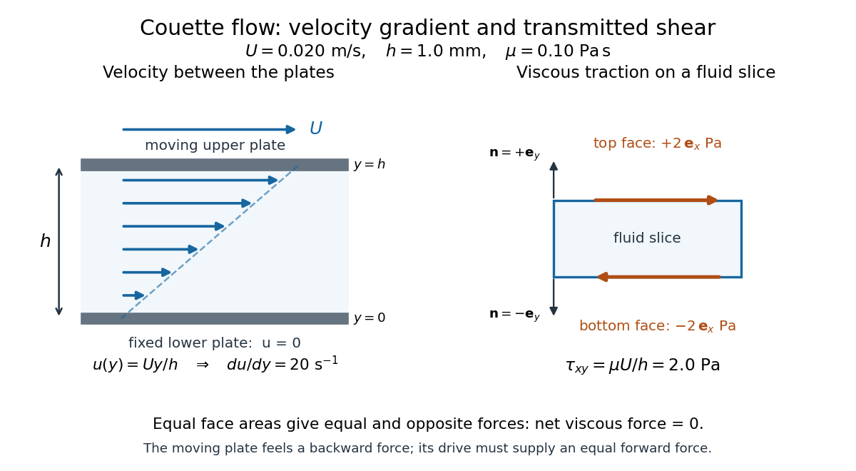
The velocity gradient matters, rather than the velocity itself. Adding the same constant velocity to both plates and the fluid leaves $du/dy$, and hence shear stress, unchanged. In uniform flow, every layer translates together and $du/dy=0$. More generally, even a nonzero velocity gradient need not generate viscous stress: solid-body rotation has zero strain-rate tensor, as the viscous stress tensor example shows. Thin gaps amplify shear stress for a fixed plate-speed difference, making dynamic viscosity useful for predicting the force needed to move lubricated surfaces.

A fluid is a material that flows under sustained shear stress and cannot maintain a static shear stress in its fluid state. Liquids and gases are the usual examples. A Newtonian fluid has deviatoric stress proportional to its rate-of-strain tensor, whereas more general fluid constitutive equations can be nonlinear or have memory. In a porous medium, the fluid occupies connected voids within a load-bearing solid framework. The important distinction is the response to a continuing tangential force: an ordinary elastic solid can settle into a fixed deformation, while an ordinary fluid continues to deform. A fluid can nevertheless be at rest when no unbalanced shear stress drives it. ^[ref]

For a worked example, place a Newtonian fluid between parallel plates separated by $h=1\mathrm{mm}$, keep the lower plate fixed and move the upper one at $U=0.10\mathrm{m}{\mathrm{s}}^{-1}$. With no-slip boundary conditions, steady flow, no imposed pressure gradient and negligible edge effects, Couette flow has $u(y)=Uy/h$. For dynamic viscosity $\mu =0.001\mathrm{Pa}\mathrm{s}$, the shear stress magnitude isThe velocity gradient describes neighbouring layers sliding at different speeds. Doubling $U$ doubles the required shear stress; maintaining the same velocity keeps producing deformation, rather than fixing a final shape. This gives viscosity a concrete meaning: resistance to a rate of motion, not a prohibition on motion.

A homologous spherical flow has velocity proportional to radius. Its velocity gradient is $q(t)I$ and its velocity divergence is $3q(t)$.

An objective spatial second-rank tensor transforms by the displayed rule under every rigid observer change $x^{\ast }=c(t)+Q(t)x$. This permits time-dependent rotations, not merely constant rotations. Cauchy stress tensor is objective because contact traction and surface normal both rotate by Q. The symmetric rate-of-strain tensor is objective because the additional observer spin in the velocity gradient is antisymmetric.

For the specified affine linear PTT fluid, perturb about the relaxed state $A=0$, $\mathbf{v}=0$. Products of $A$ with the velocity gradient and the term $\alpha (\mathrm{tr}A)A$ are second order in the perturbation. The material-advection term is also second order. The linearized equation is thereforeWith vanishing stress in the remote past, an integrating factor givesSince ${\sigma }^{\prime }=G_{0}A$, comparison with the linear viscoelastic fluid convolution yields $G(s)=G_0{e}^{-s/\tau }$ and zero-shear viscosity $G_0\tau$. The nonlinear relaxation parameter does not appear at linear order; the response is that of a Maxwell fluid.

An isotropic simple fluid has local stress determined by the deformation history of the material element. A viscometric flow is one whose relative deformation history is that of steady simple shear flow, up to rigid changes of frame. At a given element the shear rate is constant along its history, although it can differ between elements. This includes the locally simple-shear kinematics used in standard viscometric measurements.

Use the component-first velocity gradient $K_{ij}=\partial v_i/\partial x_j$. The first two Rivlin-Ericksen tensors areIn the axes of a steady shear $v_x=sy$, the relative deformation gradient over a lag $q$ is $F=I+qK$, since $K^2=0$. The material history is determined by $s$, and its tensor symmetries exclude $xz$ and $yz$ stress components. The remaining symmetric stress consists of an isotropic part, one shear component, and two independent normal-stress differences. The relevant matrices areThus $I,A_1,A_1^2,A_2$ span the allowed stress components. Material isotropy and reversal of the shear show that their scalar coefficients depend on $|s|=(A_1:A_1/2{)}^{1/2}$. Define the viscometric functions bySolving for the matrix coefficients givesThis is an exact steady-viscometric representation, rather than an assumption that the fluid is everywhere a second-order fluid. The shear viscosity $\mu$ measures the shear resistance, while ${\psi }_1$ and ${\psi }_2$ measure the first and second normal-stress differences generated by shear. Their zero-rate values are understood as limits when these exist. An isotropic pressure changes neither normal difference.

For a flow in the lubrication approximation with gap $H$, longitudinal scale $\ell \gg H$ and speed $U$, the shear-rate scale is $U/H$. The viscous shear force per unit volume scales as $\mu U/H^2$. Quadratic viscoelastic normal stresses scale as ${\psi }_i{U}^2/H^2$; their longitudinal gradients, and the comparable mixed-component corrections, contribute forces of scale ${\psi }_i{U}^2/(H^2\ell )$. Therefore the normal-stress smallness in lubrication criterion isEquivalently, the thin-gap aspect ratio must multiply the shear-based elastic parameter to give a small quantity: $(H/\ell )|{\psi }_i|\dot{\gamma }/\mu \ll 1$. Normal stresses need not themselves be smaller than the shear stress; it is their effect on the leading force balance that matters. If the flow changes on an additional short time scale $T$, the $D_t{A}_1$ term also requires $|{\psi }_1|/(\mu T)\ll 1$ for its neglect. Material coefficients should be evaluated at the characteristic shear rate.

Now take positive cylinder rotation, measure $\theta$ counterclockwise from the rightward horizontal, and let $y=r-a$ increase outward through the film. The tangent has upward component $\cos \theta$, so the tangential gravitational acceleration is $-g\cos \theta$. To leading order in $h/a$, neglect inertia and higher-order hydrostatic or capillary pressure gradients, and write $U=\Omega a$. Tangential force balance and the shear-free free surface givehenceThe wall shear stress is $-\rho gh\cos \theta$. It opposes rotation on the uphill side and assists it on the downhill side.

For a power-law fluid, ${\sigma }_{\theta y}=k|u_y{|}^{n-1}{u}_y$. Its inversion must retain the sign:Integrating with the no-slip boundary condition $u(0)=U$ yieldsThe volume flux per unit axial length is $Q={\int }_0^{h}u(y)dy$. The integrated bracket is $[(n+1)/(2n+1)]h^{(2n+1)/n}$, so the power-law coating on a rotating cylinder hasAt $\cos \theta =0$ the gravitational term vanishes by continuity. Steady mass conservation makes $Q$ independent of $\theta$.

On the uphill half, put $D=(\rho g\cos \theta /k{)}^{1/n}$ and $m=(2n+1)/n$. The local flux is $Q(h)=Uh-(D/m)h^m$, withIt has a unique maximum atA positive coating must carry the same steady flux at every angle. The tightest local bound occurs at $\cos \theta =1$, not on the downhill side, where the flux increases monotonically with thickness. ConsequentlyFor $0<Q<Q_{\max }$ the thinner positive root on the uphill side connects through $\cos \theta =0$ to the unique downhill root, giving a periodic leading-order coating profile. At the limiting flux the two uphill roots meet at $\theta =0$; it is the maximum flux of this lubrication model, with a possible limiting corner resolved by neglected higher-order effects. For $n=1$ the check is $Q_{\max }=(2/3)U\sqrt{kU/(\rho g)}$. All these conclusions require the resulting film to remain thin enough for the lubrication approximation and for the neglected normal stresses and inertia to satisfy their scaling restrictions.

With its material state fixed by a prescribed deformation history, the differential pom-pom model is a simple-fluid constitutive law. The stress depends on the local history of a material element through its molecular stretch and orientation, without gradients of that history between neighbouring elements. A differential representation does not prevent a material from being a simple fluid.

To see the history dependence explicitly, use the component-first velocity gradient $K$, so the tensor evolution is $D_{t}A=KA+A{K}^T-(A-I)/{\tau }_1$. Let $F(t,s)$ be the relative deformation gradient, satisfying ${\partial }_{t}F=K(t)F$ and $F(s,s)=I$. Along a material trajectory, an integrating factor givesThus $A$ is a functional of the local deformation history and its prepared initial state. If the initial $A$ is a positive-definite matrix, it retains that property, so $B=A/\mathrm{tr}A$ is well defined. Given this $B(t)$, the scalar stretch solves $\dot{\lambda }=r(t)\lambda +1/{\tau }_2$, where $r=B:K-1/{\tau }_2$. Its variation of constants formula again depends only on that local history:The differential pom-pom model also satisfies material frame indifference. Under an observer rotation, $A$ and $B$ transform as objective tensors, while $\lambda$ is a scalar. The extra skew part of the transformed velocity gradient has zero contraction with symmetric $B$, so the stretch equation is unchanged. The tensor evolution uses an upper-convected derivative, and the final stress transforms objectively. Initial values cannot be independently forgotten when specifying a finite-past experiment: a fully specified prepared state, such as rest, is part of the history specification.

At rest the tensor equation relaxes $A$ toward $I$ and the stretch equation relaxes $\lambda$ toward one. ThusThe equilibrium nonpressure stress $GI/3$ is isotropic and can be absorbed into the arbitrary pressure in incompressible flow.

For the linear response, put $A=I+a+O({\epsilon }^2)$, $\lambda =1+\ell +O({\epsilon }^2)$ and take the velocity gradient to be $O(\epsilon )$. The first-order tensor equation isIts matrix trace has no forcing, because incompressibility gives $\mathrm{tr}K=0$. Starting relaxed, $\mathrm{tr}a=0$. The first-order stretch equation is $D_t\ell +\ell /{\tau }_2=(I/3):K=0$, hence $\ell =0$. Consequently $B=I/3+a/3+O({\epsilon }^2)$, and its anisotropic stress is $Ga/3$. From the relaxed remote past,The linear and second-order response of the differential pom-pom model therefore hasThe stretch time ${\tau }_2$ does not enter the linear shear relaxation modulus.

For the second-order fluid constants, additionally make the slow-flow expansion: count $K$ as first order and $D_t$ as raising the order by one. IteratinggivesUsing the Rivlin-Ericksen tensor convention $A_2=D_t{A}_1+A_{1}K+K^T{A}_1$, the identityreduces this to $A=I+{\tau }_1{A}_1+{\tau }_1^2(2A_1^2-A_2)+O(3)$. Since $\mathrm{tr}{A}_2=\mathrm{tr}{A}_1^2$, normalization givesStretch first changes at second order. Its equation gives $\lambda -1={\tau }_1{\tau }_2\mathrm{tr}(A_1^2)/6+O(3)$. Multiplication by ${\lambda }^2$ therefore adds only an isotropic stress at second order; multiplying its second-order increment by the anisotropic first-order term would be third order. Absorb these isotropic corrections into $p_{\ast }$ to obtainComparison with the viscometric functions parametrization yieldsEquivalently, in $\sigma =-pI+{\mu }_0{A}_1+{\alpha }_1{A}_2+{\alpha }_2{A}_1^2$, the constants are ${\alpha }_1=-G{\tau }_1^2/3$ and ${\alpha }_2=2G{\tau }_1^2/3$. The general small-amplitude linear response above permits fast oscillation; the local second-order fluid expansion also requires the slow-flow ordering just used.

For a linear viscoelastic fluid, causal superposition givesThe relaxation modulus $G(s)$ is the stress response to a unit small step of shear strain. The equation assumes an isotropic reference state and deformations and rotations small enough over the significant memory times that nonlinear transport and strain products can be neglected. Small-amplitude motion can have high frequency; linearity does not require low frequency by itself. The infinite-past integral encodes the preceding history, rather than assuming that stress vanishes whenever the present rate vanishes.

For a small constant shear rate maintained from the remote past, the rate can be taken outside the integral. Therefore the zero-shear viscosity isprovided the kernel is integrable, with any instantaneous contribution counted fully. A nondecaying solid-like modulus would not yield a finite fluid viscosity.

To linearize the stated Oldroyd-B model, put $A=I+C$ and absorb the isotropic $G_{0}I$ into pressure. The products of the small deformation tensor C and velocity gradient are second order. Using the paper's derivative-index-first gradient convention therefore givesAn integrating factor, with the prescribed preceding history, gives $C(t)=2{\int }_0^{\infty }{e}^{-s/\tau }E(t-s)ds$. Thus the linear nonpressure stress isThe regular relaxation tail is $G_0{e}^{-s/\tau }$, while the solvent is instantaneous. Equivalently, the instantaneous solvent term in a relaxation modulus can be represented byHere the causal endpoint delta is defined by ${\int }_0^{\infty }{\delta }_{+}(s)f(s)ds=f(0)$. If instead a symmetric Dirac delta is assigned half its mass at the endpoint, the same solvent term is written $2{\mu }_0\delta (s)$. Stating the convention prevents a factor-of-two error in the viscosity; the explicit stress formula above has no such ambiguity.

In a cone-and-plate rheometer, the small-angle gap is $\alpha r$ and the local wall speed is $\Omega r$, so the shear rate is independent of radius to leading order: $g(t)=\Omega (t)/\alpha$. Write $s(t)$ for shear stress and $P(t)$ for its polymer part. The linear constitutive response isThe uniform shear stress gives torqueFor the initial steady torque T, put $s_{+}=3T/(2\pi a^3)$ and ${\mu }_p=G_0\tau$, $\mu ={\mu }_0+{\mu }_p$. The steady polymer stress is $P_{+}={\mu }_p{g}_{+}$, with $g_{+}=s_{+}/\mu$. Hence the initial angular velocity is

For $t>0$, the total stress is $s=-s_{+}$, but the polymer stress is continuous at the torque reversal. Since ${\mu }_0>0$, a finite jump in shear rate is possible even though P cannot jump. Its immediate value isEliminating P from the constant-stress equations for $t>0$ givesThe decay time is the Retardation time of an Oldroyd fluid ${\lambda }_2={\mu }_0\tau /({\mu }_0+{\mu }_p)$. Solving this first-order equation with the actual initial value yields the complete torque reversal of a linear Oldroyd fluid:In particular, $\Omega (\infty )=-{\Omega }_{+}$ but $\Omega (0^{+})$ is more negative. The stored polymer stress initially retains its old positive sign, requiring a larger negative solvent shear stress to attain the new negative total torque. This produces the backward-speed overshoot and its subsequent relaxation. Apparatus inertia would smooth the instantaneous jump, but is neglected in the question. The torque must be sufficiently small for the entire transient, including its enhanced initial rate, to remain in the linear viscoelastic regime; small pre-reversal rate alone is not sufficient when $G_0\tau /{\mu }_0$ is large.

The spin tensor $W$ is skew, and $\dot{Q}{Q}^T=W$ means $\dot{Q}=WQ$ and ${\dot{Q}}^T=-Q^{T}W$. Differentiate all factors to obtain the corotating-frame representation of a Jaumann derivative:Thus the Jaumann derivative is the ordinary derivative of the tensor components in this rotating frame.

Put $S={\sigma }^d$, $\Delta \mu ={\mu }_1-{\mu }_0$, $A=S-2{\mu }_{0}D$ and $\tilde{A}=Q^{T}AQ$, $\tilde{D}=Q^{T}DQ$. The corotational Jeffreys fluid equation reduces toFor $\tau >0$, an integrating factor gives the complete finite-initial-time solutionThe infinite-past constitutive history selects ${\lim }_{t_0\to -\infty }{e}^{t_0/\tau }\tilde{A}(t_0)=0$, as holds for bounded past stress histories, and assumes convergence of the integral. Taking that limit and rotating back provesA general initial stress would retain the displayed homogeneous term. Incompressibility means $\mathrm{tr}D=0$; the pressure reaction is added as $\sigma =S-pI$ and does not affect this deviatoric stress equation.

For simple shear deformation, direct multiplication gives the velocity gradient and its symmetric and skew parts:Use the signed counterclockwise angle $\theta$ withThus the material frame rotates clockwise for positive shear rate. This angle convention is necessary for the signs of the sine terms. Set $\delta =\theta (t)-\theta (s)$. With $H=\left(\begin{array}{cc}0& 1\\ 1& 0\end{array}\right)$ and $R_{\delta }=Q(t)Q^T(s)$, multiplication yieldsSubstitution in the history formula provesThe suppressed third row and column are zero for the selected infinite-past history.

For constant shear rate $g=\dot{\gamma }$, $2\delta =-g(t-s)$. Put $u=t-s\ge 0$. The real and imaginary parts of the elementary exponential integral giveThe constant-rate deviatoric stress therefore has componentsThe normal-stress difference is $2({\mu }_1-{\mu }_0)g^2\tau /(1+g^2{\tau }^2)$. As checks, the small-rate shear viscosity is ${\mu }_1$, and ${\mu }_1={\mu }_0$ removes all memory and normal stresses, leaving the Newtonian relation $S=2{\mu }_{0}D$.

Let $F$ be an invertible, orientation-preserving deformation gradient, with $J=\det F>0$. To prove Nanson's formula, take two reference surface tangent vectors $a,b$. Their current images are $Fa,Fb$, and their oriented area vectors are proportional to $a\times b$ and $(Fa)\times (Fb)$. For every vector $c$, the scalar triple product givesThus $F^T[(Fa)\times (Fb)]=J(a\times b)$, andThis proof also identifies the area transformation as the cofactor of $F$, rather than a transformation by $F$ itself.

Use the paper's material-index-first nominal stress tensor $P_{Ii}$. Equality of force on the same material surface in its two configurations gives $P_{Ii}d{S}_{0I}={\sigma }_{ji}d{S}_j$. Substitute the area transformation to obtainHere $\tau$ is the Kirchhoff stress tensor. With symmetric Cauchy stress tensor, the matrix forms are $P=J{F}^{-1}\sigma$ and $\tau =FP$. This $P$ is the transpose of the first Piola-Kirchhoff stress tensor; keeping the index convention prevents a spurious transpose later.

For the velocity gradient $L=\dot{F}{F}^{-1}$, let $D=(L+L^T)/2$ be the rate-of-strain tensor. Then the reference-volume mechanical power isThe last step uses stress symmetry, as supplied by angular-momentum balance in an ordinary continuum without couple stresses: a symmetric tensor has zero contraction with the skew part of $L$.

By work-conjugate stress and strain, a pair $(T,E)$ must satisfy $T:\dot{E}=\tau :D$ for every deformation rate, with both sides measured per reference volume. For the Green-Lagrange strain tensor, set $C=F^{T}F$ and calculateCyclically rearranging the contraction shows $T^{(2)}:{\dot{E}}^{(2)}=(F{T}^{(2)}{F}^T):D$. Hence the symmetric conjugate isthe second Piola-Kirchhoff stress tensor.

The inverse right Cauchy-Green strain is $E^{(-2)}=(I-C^{-1})/2$, because $C^{-1}=F^{-1}{F}^{-T}$. Differentiating $C{C}^{-1}=I$ givesConsequently $T^{(-2)}:{\dot{E}}^{(-2)}=(F^{-T}{T}^{(-2)}{F}^{-1}):D$, andThe two stress measures have a geometric interpretation in the convected coordinate net. Its basis vectors are $g_I=F{e}_I$ and its reciprocal basis is $g^I=F^{-T}{e}_I$. The entries of $T^{(2)}$ are the contravariant components in $\tau =T_{IJ}^{(2)}{g}_I\otimes g_J$, whereas $T_{IJ}^{(-2)}=g_I\cdot \tau g_J$ are the covariant components, equivalently $\tau =T_{IJ}^{(-2)}{g}^I\otimes g^J$. They describe the same spatial Kirchhoff stress tensor in a deforming, generally nonorthonormal coordinate net.

Differentiate the pulled-back Kirchhoff stress tensor $T=F^T\tau F$, using the velocity gradient convention $L=\dot{F}{F}^{-1}$:Thus the lower-convected stress pull-back givesFor an explicit objective time derivative check, superpose $x^{\ast }=Q(t)x+c(t)$, with $Q^{T}Q=I$ and $\Omega =\dot{Q}{Q}^T$ skew. Then ${\tau }^{\ast }=Q\tau Q^T$ and $L^{\ast }=QL{Q}^T+\Omega$, whereasThe additional terms in $(L^{\ast }{)}^T{\tau }^{\ast }+{\tau }^{\ast }{L}^{\ast }$ are $-\Omega {\tau }^{\ast }+{\tau }^{\ast }\Omega$. They cancel the extra material-derivative terms, proving $\boxed{{\mathcal{D}}_l{\tau }^{\ast }=Q({\mathcal{D}}_l\tau )Q^T}$. The translation has no effect on a stress or velocity gradient.

For the incompressible Oldroyd-A model, avoid using the same symbol for a stress tensor and its relaxation time by referring to $\tau >0$ below only as the scalar relaxation time. Define $S={\sigma }^d-2{\mu }_{r}D$. The constitutive equation becomesBy the pull-back identity, $A=F^{T}SF$ satisfiesAn integrating factor givesPush forward by $F(t{)}^{-T}$ and $F(t{)}^{-1}$. For a convergent, fading remote-past history with the transported homogeneous term tending to zero as $t_0\to -\infty$, this proves the fading-memory representation of the Oldroyd-A model:For arbitrary finite-time initial data retain $e^{-(t-t_0)/\tau }F(t{)}^{-T}A(t_0)F(t{)}^{-1}$. Thus the printed integral-only expression incorporates an initial-memory condition; it is not an unconditional replacement for all initial-value solutions.