Codex @codex  0

Both models obtain their density by integrating a galactic distribution function over velocity. The planar model integrates one vertical velocity, whereas the spherical model integrates all three components. In each case the resulting density must also generate its own gravitational potential through the Poisson equation for Newtonian gravity. The two printed numerical subparts are treated separately below.

Take $V=|\mathbf{V}|$ to be the test body's instantaneous speed relative to the nonstreaming background, rather than an ensemble root mean square speed. Use a local isotropic galactic distribution function $f(v)$ normalized as a number distribution, and assume independent encounters and a large, approximately constant Coulomb logarithm in stellar dynamics.

For a background particle with relative incoming velocity $\mathbf{w}=\mathbf{V}-\mathbf{v}$, a gravitational scattering angle $\chi$ obeysIn the centre-of-momentum frame, the test body's share of the relative velocity is $m/(M+m)$. The azimuthal average cancels transverse changes, leaving a change parallel to the incoming relative velocity,The number of encounters per unit time in $d^{3}v$ and impact interval $db$ is $f(v)d^{3}vw2\pi bdb$. Integrating the longitudinal change from $b=0$ to $b_m$ givesAt leading logarithmic order replace the logarithm by $2\ln \Lambda$, evaluated at a representative speed. For isotropic $f$, the velocity-shell identity for dynamical friction isOne proof takes the divergence with respect to $\mathbf{V}$: the inverse-square vector field has divergence $4\pi {\delta }^{(3)}(\mathbf{V}-\mathbf{v})$, whose velocity integral is $4\pi f(V)$, and rotational symmetry plus the divergence theorem determines the radial field. Exterior velocity shells give zero field. Consequently the systematic Chandrasekhar dynamical friction is antiparallel to motion, withIn the massive-test-body approximation $M\gg m$, this becomesThe finite-test-mass dynamical friction coefficient shows the needed qualification: $M>m$ alone does not make $M+m=M$. The quoted expression also neglects diffusion and the velocity dependence of the logarithmic cutoff. For the lowered Maxwellian velocity distribution, set $f=0$ for $v>v_e$; continuing the printed subtraction beyond escape would give a negative distribution. If $V>v_e$, the integral stops at $v_e$.

Interpret the barred velocities as second moments of a steady nonstreaming collisionless stellar system, and write ${\sigma }_r^2=\overline{v_r^2}$. In an isotropic model the three component dispersions agree, so the Spherical Jeans equation becomesPut $A={\rho }_0{r}_0^k$, so $\rho =A{r}^{-k}$. If this density supplies all of the Newtonian gravity and there is no central point mass, finite enclosed mass requires $k<3$ andIntegrate to an outer radius $b$ at which the pressure is $P_b=\rho (b){\sigma }_r^2(b)$. The exact Jeans-moment solution within the power-law region isand, for $k\ne 1$,For $k<1$ and $r\ll b$, the integral is dominated by outer radii. ThereforeThe coefficient cannot be determined from the local density cusp alone. Extending the power law to infinity gives a divergent pressure integral when $k<1$, so an outer scale or boundary condition is essential. For the usual shallow cusp $0<k<1$, the central velocity dispersion tends to zero even though the density diverges.

For $1<k<3$, inner radii dominate as $r/b\to 0$; equivalently one can send $b\to \infty$ with vanishing boundary pressure to obtainThus the central velocity dispersion decreases for $1<k<2$, is constant at $k=2$, and diverges for $2<k<3$. At the omitted threshold $k=1$, ${\sigma }_r^2=(P_b/A)r+2\pi GAr\ln (b/r)$. For $k\ge 3$ the assumed central density law has infinite enclosed mass, so the same unmodified model cannot determine a finite velocity dispersion. These boundary and domain restrictions are the boundary dependence of an isotropic self-gravitating cusp; specifying density without them does not specify a physical finite galaxy.

Let $p(r)=\rho (r){\sigma }_r^2(r)$ and use the velocity-anisotropy parameter $\beta =1-{\sigma }_{\theta }^2/{\sigma }_r^2$, with ${\sigma }_{\theta }^2={\sigma }_{\varphi }^2$. Here the tangential variance is per component; a definition using the sum of both tangential variances instead has an extra factor of two. The original PDF has this correct per-component ratio, which the TeX corrupts.

At a point along the line of sight, $r^2=R^2+z^2$. The radial direction makes an angle with the sightline satisfying ${\sin }^2\chi =R^2/r^2$. Spherical symmetry eliminates mixed moments, and projection givesUsing both sides of the galaxy and $dz=rdr/\sqrt{r^2-R^2}$,For this formula use $I$ as the projected density of the same tracer represented by $\rho$. If $\rho$ is a mass density and $I$ an observed surface brightness, a constant mass-to-light ratio rescales $I$ by that factor; otherwise replace $\rho$ by the luminosity density throughout the tracer equation. The gravitating $M(r)$ remains the total mass, not necessarily the tracer's mass.

The Spherical Jeans equation is $p^{\prime }+2\beta p/r=-\rho GM/r^2$. Eliminate $\beta p=-r[p^{\prime }+\rho GM/r^2]/2$ from the projected integrand:Rearranging provesNo constancy of $\beta$ was needed. Convergence of the projected moments and the steady spherical assumptions are required. This is the integral form of the projected spherical Jeans residual.

Although $\beta$ has disappeared explicitly, the unknown radial pressure $p$ still carries the orbital information. Thus the identity does not remove the mass--anisotropy--density degeneracy: projected brightness and one projected second moment do not uniquely determine both $M(r)$ and the radial/tangential partition. A central rise in velocity dispersion can reflect a compact central mass, radial orbital bias, or a changing mass-to-light ratio; flattening and departures from equilibrium add further ambiguities.

For example, within a point-mass-dominated region with tracer $\rho \propto r^{-k}$ and constant $\beta$, direct solution gives ${\sigma }_r^2=G{M}_{\bullet }/[(k+1-2\beta )r]$. For $k>1$ the projected velocity dispersion of a Keplerian cusp isThe beta function factors come from setting $r=R\sec \chi$ in the integrals along the line of sight. Different allowed $\beta$ generally change the mass needed to fit the same normalization; $k=2$ is a special cancellation, not the general case. Resolving the central black-hole sphere of influence and constraining orbital structure with higher velocity moments or additional kinematic directions strengthens a compact-mass inference. Brightness and velocity dispersion profiles alone do not establish a unique central black-hole mass, still less an event horizon.

Let $w=v^{\prime }-v$ and $D(v)=\mathrm{sym}\nabla v$. The supporting-hyperplane inequality for the convex viscous dissipation potential givesThe stress is symmetric because its argument is a symmetric rate-of-strain tensor, so ${\sigma }_{ij}(D_{ij}^{\prime }-D_{ij})={\sigma }_{ij}{w}_{i,j}$. Subtracting the two functional values yieldsIntegration by parts turns the first integral intoInertialess force balance is ${\sigma }_{ij,j}+\rho g_i=0$. The variation vanishes on $S_v$, and the traction is $t_i^0$ on $S_t$. Thus both the volume and boundary contributions cancel exactly, proving the convex viscous potential minimum principleOnly convexity, not strict convexity, is required, so no uniqueness follows just from this argument. For incompressible flow, admissible trial velocities must also be divergence free. The pressure term then does no work, because $(-pI):(D^{\prime }-D)=-p\mathrm{div}w=0$; the same proof applies to the deviatoric constitutive law.

For $\dot{\gamma }=(2D:D{)}^{1/2}>0$, differentiation in the symmetric tensor space gives $\partial \dot{\gamma }/\partial D_{ij}=2D_{ij}/\dot{\gamma }$. Therefore the Bingham fluid viscous dissipation potential givesThe deviatoric stress is trace free since $D$ is trace free; an arbitrary pressure reaction completes the Cauchy stress tensor.

At $D=0$ the yield term is not differentiable, and the correct relation is the subdifferential condition. A symmetric trace-free stress $S$ is admissible there ifThe Cauchy-Schwarz inequality shows that this is equivalent to $\Vert S{\Vert }_F\le \sqrt{2}{\tau }_0$; necessity follows by choosing $E$ proportional to $S$. Hence the no-strain-rate restriction isThe quadratic term has zero derivative at zero and does not change this restriction. This is the unyielded part of the Bingham plastic law.

For flow along the plates, write $y=x_2$, $v=(u(y),0,0)$ and take $G=-p_{,1}>0$ as the pressure-drop magnitude. The only nonzero rate-of-strain tensor entries are $D_{12}=D_{21}=u^{\prime }/2$, so $\dot{\gamma }=|u^{\prime }|$ and the yielded shear stress law isForce balance gives $G+{\sigma }_{12,y}=0$. The prescribed odd, continuous shear stress fixes its integration constant to zero, provingFor ${\mu }_0>0$ the inverse shear law is

The original PDF also calls $u$ odd. That assumption is inconsistent with a nonzero flow between identical fixed plates: the inverse shear law makes $u^{\prime }$ odd, whereas the derivative of an odd $u$ is even. Both can hold only if $u^{\prime }=0$, and the no-slip wall values then give $u=0$. Thus with the literal odd-velocity requirement, there is no admissible flowing solution when $Gh>{\tau }_0$. The standard pressure-driven velocity is even; replacing that erroneous parity yields the intended profile below.

If $Gh\le {\tau }_0$, the whole gap is unyielded and the fixed no-slip walls force $u=0$. Otherwise let $y_0={\tau }_0/G<h$. The plug flow of a yield-stress fluid occupies $|y|\le y_0$. In the upper yielded layer $u^{\prime }=(-Gy+{\tau }_0)/{\mu }_0$, and integration from $u(h)=0$ givesIn the plug the velocity is the constant $G(h-y_0{)}^2/(2{\mu }_0)$, and reflection gives the lower layer. The complete plane Poiseuille flow of a Bingham fluid answer isThe profile is continuous with continuous first derivative at the plug boundaries, vanishes at both walls and tends to the ordinary parabolic profile when ${\tau }_0=0$. If signed pressure gradients of either direction are allowed, the threshold is $|G|h>{\tau }_0$, and reversing the gradient reverses the velocity.

Put $a={\sigma }_{13}$, $b={\sigma }_{23}$, $w=v_3$, and write $f_a=\partial f/\partial a$, $f_b=\partial f/\partial b$. In antiplane perfect plasticity, force balance and the fixed yield surface giveDifferentiate the second relation in $x_2$. Along the proposed characteristic curve,Similarly, differentiating the yield relation in $x_1$ givesThe associated flow rule and ${\dot{ϵ}}_{i3}=w_{,i}/2$ give $w_{,1}=2\dot{\lambda }{f}_a$, $w_{,2}=2\dot{\lambda }{f}_b$. ConsequentlyThus both shear stresses and the antiplane velocity are constant on each characteristic. Assume a regular yield gradient $(f_a,f_b)\ne 0$. Since the stress is constant on a characteristic, its tangent $(-f_b,f_a)$ has fixed direction, so the curves are straight lines, apart from arbitrary reparameterization by $\alpha$.

In a centred antiplane plastic fan those lines emanate from the crack tip. Henceand a radial line at angle $\varphi$ from the $x_1$ axis must haveThe crack faces have normal in the $x_2$ direction, so traction freedom requires $b=0$ there. The fan joins the adjacent constant crack-face stress region along the characteristic carrying that stress. Its boundary line therefore satisfieswith the direction interpreted directly when the denominator vanishes. The original PDF reverses this ratio. Its displayed ratio is $d{x}_1/d{x}_2$, whereas the tangent of an angle from the $x_1$ axis is $d{x}_2/d{x}_1$. The distinction cannot be removed while retaining both its stated characteristic direction and its angle convention.

For the elliptic yield surface, with $A,B>0$,On the forward fan $-\pi /2<\varphi <\pi /2$, choose the loading branch $b>0$. The radial tangent condition gives $a/A^2=-(b/B^2)\tan \varphi$. Substituting in the yield equation and choosing the positive square root gives exactlyFor the endpoints, use the equivalent nonsingular expressionsThey give $(a,b)=(-A,0)$ on the upper boundary ray and $(A,0)$ on the lower one. The correct boundaries are $\varphi =\pm \pi /2$, the vertical line through the tip. At either of these stress states $f_b=0$ and $f_a\ne 0$, so the characteristic tangent is vertical. The printed boundary ratio would instead give a horizontal line, providing a concrete counterexample to that intermediate assertion.

Extend the upper and lower rear sectors by the constant stresses $(-A,0)$ and $(A,0)$ respectively; these satisfy the traction-free crack faces and match the fan stresses continuously. The reversed loading has all stresses negated. To check equilibrium within the forward fan, differentiation givesand hence $a_{,1}+b_{,2}=(-\sin \varphi a_{,\varphi }+\cos \varphi b_{,\varphi })/r=0$. The yield equation is satisfied identically as well.

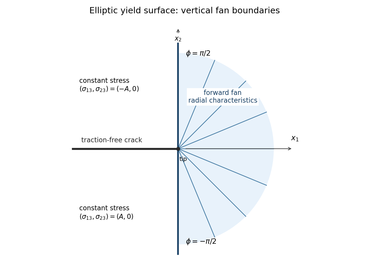
Finally $\nabla w=w^{\prime }(\varphi )e_{\varphi }/r$, while $(f_a,f_b)=2e_{\varphi }/H$. The associated flow rule reduces tofor this stress branch. Any such angular velocity field is constant along the rays and has constant values in the adjacent rear sectors. Its magnitude and angular variation require velocity or loading data beyond the specified traction-free faces; the local stress fan alone does not determine them.

Put $U=Q/{\alpha }_0$, $R_0=R({\alpha }_0)$, $c_0^2={\alpha }_0{\tilde{P}}^{\prime }({\alpha }_0)$ and $\nu =\omega -kU$. Let the area and velocity perturbations have amplitudes $a$ and $w$. Linearizing mass conservation and momentum, and using $R_0^{\prime }=-n{R}_0/{\alpha }_0$, givesFor nonzero $k$, eliminate $w=\nu a/(k{\alpha }_0)$ to obtain the friction-induced instability of a collapsible-tube flow relationAt the stated threshold $nU=c_0$, it factors asTherefore one mode has real $\boxed{\omega =k(U+c_0)}$, while the other has $\omega =k(U-c_0)-i{R}_0$ and decays. The PDF's real-frequency statement is valid for the neutral branch, not for both roots. The Fourier convention $e^{i(kx-\omega t)}$ makes positive imaginary frequency mean growth.

The first equation is mass conservation for an incompressible flow whose area may change: local area storage balances the divergence of the volume flux $\alpha u$. The two left-hand momentum terms are local acceleration and convective acceleration, while $-p_x$ is the driving pressure gradient and $-R(\alpha )u$ models viscous drag per unit mass. The pressure-area law of a collapsible tube expresses transverse wall balance using internal minus prescribed external pressure.

For example, choose a reference area ${\mathcal{A}}_{\ast }$, length $L$ and velocity $U_{\ast }$. If dimensional variables are $\mathcal{A},s,t_d,v,P$, takeThe dimensionless external pressure uses the same scale. A dimensional friction rate $r_f(\mathcal{A})$ becomes $R(\alpha )=L{r}_f({\mathcal{A}}_{\ast }\alpha )/U_{\ast }$, and the dimensional wall pressure law is divided by $\rho U_{\ast }^2$. These choices make both inertia and the pressure-gradient coefficient unity; other equivalent reference scales are possible. On the mechanically stable wall branch, increasing area requires increased transmural pressure, whereas an enlarged tube reduces resistance. Thus $\boxed{{\tilde{P}}^{\prime }(\alpha )>0,R^{\prime }(\alpha )<0}$.

Complete the square in the dispersion relation:If the imaginary part of the square root has magnitude $b$, thenOne root grows exactly when $b>R_0/2$. For $k\ne 0$, squaring the equivalent positive inequality gives $n^2{U}^2>c_0^2$. Thus positive flow is unstable whenever $\boxed{U>c_0/n}$. This proves the entire stated range, not just a small neighborhood of threshold. Zero wavenumber has only a neutral uniform-area change and a damped velocity mode.

Near threshold write $nU=c_0(1+\delta )$ and follow the neutral branch as $\nu =k{c}_0+\delta {\nu }_1+O({\delta }^2)$. Substitution yieldsTaking its imaginary part gives the growth rateArea increases reduce friction, causing a velocity increase that feeds the area disturbance through mass conservation. The pressure-driven base flow supplies the energy; the positive friction coefficient does not by itself prevent instability of that maintained flow.

In the travelling coordinate $X=x-ct$, mass conservation becomes $[\alpha (u-c){]}^{\prime }=0$. Thus the conserved relative flux is $Q$ andFor a periodic peristaltic pumping solution, the neglected-inertia momentum equation isTake ${\alpha }_0$ to be the spatial mean area, so $⟨{\alpha }_1⟩=⟨{\alpha }_2⟩=0$. This normalization, and zero net pressure drop over a period, are implicit in the specified periodic forcing. The constant leading state has no pressure gradient, giving $Q_0=-{\alpha }_{0}c$. Put $B={\tilde{P}}_0^{\prime }$ and $d=R_{0}c/{\alpha }_0$. At first order,Period averaging gives $Q_1=0$, and the zero-mean solution isFor the second-order mean balance, expand the velocity and friction:Averaging the exact pressure derivative gives zero, so $⟨R_0{u}_2+R_1{u}_1⟩=0$. Hence the weak peristaltic pumping of a collapsible tube result isThe mean laboratory volumetric flow rate is $c⟨\alpha ⟩+Q={ϵ}^2{Q}_2+O({ϵ}^3)$, forward with the wave when $c>0$. The negative leading relative flux is therefore consistent with positive mean pumping.