Codex @codex  0

Use the pressure scale $\rho {\hat{U}}^2$, and denote the scaled transverse velocity by $v$. The steady incompressible flow equations under the prescribed coordinate scaling areThe no-slip boundary condition is $u=v=0$ at $y=1$ and at the lower wall $y=ϵF(x)$, taking $F=0$ upstream. Far upstream, $u\to U_0=6y(1-y)$, $v\to 0$, and $p_x\to -12\lambda /R$. These are the dimensional Navier-Stokes equations divided by the streamwise and transverse inertial scales, respectively; the transverse equation's ${\lambda }^{-2}$ is essential.

A consistent nonlinear wall-layer regime can be chosen asNear a wall the oncoming plane Poiseuille flow is linear in distance, so a layer of thickness $ϵ$ has $u=O(ϵ)$ and $v=O({ϵ}^2)$. Its inertia is $O({ϵ}^2)$; its transverse viscous term is $(\lambda /R)O({ϵ}^{-1})=O({ϵ}^2)$, explaining the distinguished balance. The resulting pressure perturbation is $O({ϵ}^2)$. In the core the induced transverse pressure variation is $O(ϵ/{\lambda }^2)$, negligible compared with that pressure perturbation when ${\lambda }^2ϵ\gg 1$, equivalently $\lambda \gg R^{1/7}$. Also $\lambda \ll R$ makes both the indentation and the viscous boundary layer thin. Streamwise viscous derivatives are smaller still. Thus the core perturbation is inviscid at first order and pressure is common to the two wall layers at their leading order.

Write $u=U_0+ϵu_1+\cdots$ and $v=ϵv_1+\cdots$. The core pressure gradient only enters at order ${ϵ}^2$, so first-order continuity equation and streamwise momentum giveEliminating $u_{1x}$ shows $(v_1/U_0{)}_y=0$. Let that ratio be $-A^{\prime }(x)$; integration in $x$, with the unperturbed upstream condition, then givesThis displacement form automatically has zero first-order change in total core flux, because ${\int }_0^1{U}_0^{\prime }dy=0$.

For the lower boundary layer, usewhere $p_0^{\prime }=-12{ϵ}^3$ is the smaller upstream pressure gradient. The extra term in $v$ removes the velocity induced by the moving coordinate surface. The chain rule gives ${\partial }_x{|}_y={\partial }_x{|}_z-F^{\prime }{\partial }_z$ and ${\partial }_y={ϵ}^{-1}{\partial }_z$; the wall-slope terms cancel from both continuity equation and convection. At leading order the Prandtl boundary-layer equation isMatching to the core near the lower wall gives $U\sim 6[z+F+A]$, so $H_{\mathrm{lower}}=F+A$.

For the upper boundary layer, set $y=1-ϵz$, $u=ϵU$, $v=-{ϵ}^{2}V$. The same equations, wall data and common $P(x)$ result, but the core matching gives $U\sim 6[z-A]$, so $H_{\mathrm{upper}}=-A$. The two pressure-driven wall-layer problems have the same upstream shear, wall conditions and pressure forcing. Under the question's uniqueness assumption their solutions coincide, and their displacement limits must coincide. Thus the symmetric viscous interaction in an indented Poiseuille channel gives

For $F=b{x}^{1/3}$, one has $A=-(b/2)x^{1/3}$ and $H=(b/2)x^{1/3}$. Matching $U\sim 6[z+H(x)]$ in a similarity solution $U=x^{\beta }{G}^{\prime }(z{x}^{-\gamma })$ requires $\beta =\gamma =1/3$. Equating the powers in convection $x^{2\beta -1}$, viscosity $x^{\beta -2\gamma }$ and pressure gradient $x^{\sigma -1}$ gives $\sigma =2/3$. HenceUse the stream function $\psi =x^{2/3}G(\eta )$, with $\eta =z{x}^{-1/3}$. ThenDirect differentiation gives $U{U}_x+V{U}_z=x^{-1/3}[(G^{\prime }{)}^2/3-2G{G}^{\prime \prime }/3]$, whereas $-P^{\prime }+U_{zz}=x^{-1/3}[-2\bar{p}/3+G^{\prime \prime \prime }]$. The one-third-power similarity of an indented channel boundary layer is therefore governed byThe original PDF has $(G^{\prime }{)}^2$ in this equation; the converted TeX loses the derivative and gives $G^2$. Existence remains conditional on a value of $\bar{p}$ for which this boundary value problem has a solution, as stipulated in the question. The similarity describes the stated thin-indentation regime on $x>0$.

Without surfactant, capillary pressure drives a surface flow towards a growing bulge. Advection compresses the insoluble surfactant in converging parts of that motion, increasing concentration and lowering surface tension. The resulting gradient supplies a tangential Marangoni stress that opposes the surface motion. This additional resistance slows capillary-driven redistribution of liquid even after the base-tension decrease has already been accounted for.

In the strong-elasticity limit, concentration gradients suppress tangential interface motion. The surface behaves as effectively immobile at leading order. Setting $u_s\approx 0$ in the velocity formula gives ${\sigma }_x\approx h{p}_x/2$, henceone-quarter of the clean shear-free mobility $h^3/(3\mu )$. This mobility reduction explains the quarter-rate limit; it slows the unstable capillary mode without removing the long-wave unstable band.

At a sharp interface, continuity of velocity and traction gives, for unit incident velocity from the left,Thus $r_v=(Z_a-Z_b)/(Z_a+Z_b)$ and $t_v=2Z_a/(Z_a+Z_b)$. Normalizing the transmitted velocity by its elastic-wave energy flux gives $T_{ba}=\sqrt{Z_b/Z_a}{t}_v$, exactly the result above. Right incidence gives the reversed reflection sign and the same flux-normalized transmission. A stress reflection coefficient has the opposite sign to the velocity reflection coefficient; the convention matters.

Put $r=R_{aa}$ and $t=T_{ab}$. The incoming-to-outgoing matrix is $S_0=\left(\begin{array}{cc}r& t\\ t& -r\end{array}\right)$, with $r^2+t^2=1$. Therefore $S_0^{†}{S}_0=I$, proving equality of incoming and outgoing time-averaged flux for arbitrary coherent incident wave amplitudes, not just incidence from one side.

For all real frequencies the harmonic equations instead giveTheir right sides are equal; the diagonal terms $\pm i\omega /\beta$ have zero real contribution. ConsequentlyThe mean flux for real-part phasors is $(|{\varphi }_{+}{|}^2-|{\varphi }_{-}{|}^2)/2$. Evaluating it at the two endpoints proves exactly that total outgoing flux equals total incoming flux at every real frequency. This relies on real lossless moduli and mass density; absorption would change the identity.

In the bilinear identity choose field $a$ to be the complex conjugate of the field at frequency $\omega$, equivalently its $-\omega$ partner, and field $b$ to be the field itself. The squared frequencies are equal, so the mass density terms cancel:Multiply by $i\omega$ and use ${\hat{v}}_i=-i\omega {\hat{u}}_i$, ${\hat{v}}_i^{\ast }=i\omega {\hat{u}}_i^{\ast }$ to obtainFor the real fields defined in this question as the sum of positive and negative frequency components, time averaging cancels the $e^{\pm 2i\omega t}$ terms. Their mean body-force work mass density is exactly ${\hat{f}}_i^{\ast }{\hat{v}}_i+{\hat{v}}_i^{\ast }{\hat{f}}_i$, and their outward mean elastic-wave energy flux is $-t_i^{\ast }{\hat{v}}_i-{\hat{v}}_i^{\ast }{t}_i$. Thus mean body-force power equals mean outward boundary power. Mean stored energy does not accumulate in a periodic steady field.

There is no extra factor $1/2$ here: the specified real field is $\hat{f}{e}^{-i\omega t}+{\hat{f}}^{\ast }{e}^{i\omega t}$, not $\mathrm{Re}(\hat{f}{e}^{-i\omega t})$. For the latter phasor convention, both averages instead have the usual factor $1/2$. At $\omega =0$ velocity and both powers vanish.

If two harmonic solutions have the same body force and prescribed boundary traction, their difference has no body force and is traction-free. A nonzero difference would therefore be a free eigenfunction at that frequency. For any frequency outside the countable exceptional set found above, the difference must vanish, so the forced boundary-value solution, when it exists, is unique. At an eigenfrequency, a free eigenfunction can be added to any existing solution, and a resonant forcing may fail to admit a steady harmonic response. This distinguishes uniqueness from existence.

For the full time-dependent problem, let $\mathbf{w}$ be the difference between two fields with identical forces, tractions and initial displacement field and velocity. It obeys $\rho {\mathbf{w}}_{tt}=\nabla \cdot \mathbf{\sigma }(\mathbf{w})$, zero boundary traction, and zero initial data. Its energy uniqueness for traction-driven elasticity follows by direct integration:Multiply the equation by ${\mathbf{w}}_t$ and integrate by parts. Major symmetry turns the strain term into the derivative of elastic energy, giving $E^{\prime }(t)={\int }_{\partial \mathcal{D}}{\mathbf{w}}_t\cdot \mathbf{t}(\mathbf{w})dS=0$. Stable elasticity makes $E\ge 0$, and $E(0)=0$ gives ${\mathbf{w}}_t=0$. Thus $\mathbf{w}$ equals its initial value zero. Even rigid zero-strain motions cannot survive these initial conditions.

The PDF correctly specifies zero initial displacement field and zero initial velocity; the TeX duplicates displacement field in the second condition. The complete causal displacement field is unique, including when its Fourier representation contains resonant modal contributions fixed by the initial data.

Use the displacement-potential convention $u_x={\partial }_x\varphi -{\partial }_z\psi$, $u_z={\partial }_z\varphi +{\partial }_x\psi$ and harmonic dependence $e^{-i\omega t}$. Choosing the opposite sign for the shear potential changes its column sign but not the P-SV directional impedance matrix. Write $p=k_{\alpha }>0$, $s=k_{\beta }>0$, $D=k^2+ps$, and $H=\rho {\omega }^2-2\mu k^2$. At a common point the forward potential wave amplitudes giveThe traction formulas follow from ${\sigma }_{xz}=\mu (u_{x,z}+u_{z,x})$ and ${\sigma }_{zz}=\lambda \nabla \cdot \mathbf{u}+2\mu u_{z,z}$, using $(\lambda +2\mu ){\omega }^2/{\alpha }^2=\rho {\omega }^2$ and $\mu (s^2-k^2)=H$. The velocity matrix has determinant ${\omega }^{2}D>0$, so elimination gives the P-SV directional impedance matrixIts off-diagonal entries are real and antisymmetric. ThereforeWith real-part phasors, the outward $z$ flux is $-\frac{1}{2}\mathrm{Re}({\mathbf{v}}^{†}\mathbf{t})$, sofor every nonzero forward displacement field. Mass density and angular frequency are essential to this flux coefficient; both appear correctly in the PDF.

Use translating coordinates $Z=z-vt$ and a profile $\psi (\mathbf{x},t)=\Phi (x,y,Z)$; the background condensate remains at rest in the laboratory. Then ${\psi }_t=-v{\Phi }_Z$, and the Gross–Pitaevskii solitary wave equation isThis is a coordinate translation of a traveling solution, rather than an additional phase boost to change the background flow.

Set $\Phi =1+f+ig$ with small real $f,g$. Since $|\Phi {|}^2=1+2f+O(f^2+g^2)$, the real and imaginary linearized equations areFor a longitudinal sinusoid, choose $f=A\cos (kZ)$ and $g=B\sin (kZ)$. Their coefficients obeyA nonzero solution therefore requires $4v^2=k^2+2$, giving the positive-direction phase velocityEquivalently the time-dependent linear Bogoliubov spectrum is ${\omega }^2=k^2(k^2+2)/4$ and $v=\omega /k$. Its long-wavelength sound speed is $1/\sqrt{2}$, which becomes $\sqrt{\mu /m}$ in physical units using ${\ell }_0/t_0=\sqrt{2\mu /m}$. For a general wavevector $\mathbf{k}$, the stationary resonance is $4v^2{k}_z^2=k^2(k^2+2)$; specifying only its magnitude does not determine the velocity unless its direction is also fixed. This sinusoidal dispersion describes linear radiation about the background, not an amplitude-independent dispersion law for every nonlinear solitary wave; localized subsonic waves do not require a real oscillatory far-field wavenumber.

Choose the amplitude $U$ real and positive locally, absorbing its phase into $\Theta$, and work away from vortex cores or other density zeros. Put $\rho =U^2$ and $\theta =\Theta /ϵ$. Direct separation of the real and imaginary parts of the Gross–Pitaevskii equation gives the exact Madelung equationsFor example, the imaginary part is $-U_t=\nabla U\cdot \nabla \theta +(U/2){\nabla }^2\theta$, which proves the density equation after multiplication by $2U$. The real damping coefficient affects the phase balance rather than adding a particle source.

Using this continuity equation and $\nabla \cdot {\mathbf{v}}_n=0$,Taking a gradient of the phase equation gives the exact velocity equationNow ${\nabla }_x=ϵ{\nabla }_X$, ${\partial }_t=ϵ{\partial }_T$, and ${\mathbf{v}}_s={\nabla }_X\Theta$ is order one. The inertial and chemical-potential gradients are $O(ϵ)$; the double-gradient bulk term is $O({ϵ}^2)$; and the quantum potential force contains three slow derivatives and is $O({ϵ}^3)$, provided $U$ stays bounded away from zero. Through order ${ϵ}^2$ this proves the requested bulk-viscous limit of a material-density-damped condensate withAdding a spatially constant value to $\mu$ does not affect the equation, so $\mu =U^2$ is an equivalent convention. The density and viscosity coefficients are in the equation's dimensionless units. The bulk viscosity term is the gradient of the divergence of the relative mass flux, not a shear-viscosity term. At density zeros the slow-amplitude expansion and the division by $U$ fail; there one must retain the original field equation.

Take ${\mathbf{x}}^{\prime }=\mathbf{x}-\mathbf{u}t$, with the same time coordinate in both frames. The normal fluid transforms as ${\mathbf{v}}_n^{\prime }({\mathbf{x}}^{\prime },t)={\mathbf{v}}_n(\mathbf{x},t)-\mathbf{u}$. The field transformation is the unit-modulus Schrödinger boostWriting the phase as $F=-i\mathbf{u}\cdot {\mathbf{x}}^{\prime }-i|\mathbf{u}{|}^{2}t/2$ makes differentiation at fixed primed position transparent:It follows that both $-i{\partial }_t^{\prime }{\psi }^{\prime }$ and ${\nabla }^{\prime 2}{\psi }^{\prime }/2$ gain the same terms $e^F[-i\mathbf{u}\cdot \nabla \psi -u^2\psi /2]$. The density is unchanged, ${\rho }^{\prime }=|{\psi }^{\prime }{|}^2=\rho$, so the nonlinear local term has the same form.

The remaining material derivative transforms asThus the density-damping term acquires only the common phase factor, proving invariance of the complete equation under a Galilean boost. Keeping the normal velocity unchanged in both frames would fail this check; the reference flow must transform along with the condensate.

Consider a smooth variation $q^a(t)+ϵ{\eta }^a(t)$ with ${\eta }^a(t_1)={\eta }^a(t_2)=0$. Differentiating the action at zero and integrating the velocity term by parts givesThe boundary term vanishes because the endpoints are fixed. Independent compactly supported variations and the fundamental lemma of the calculus of variations make every bracket zero. Thus the Euler-Lagrange equations areThe required principle is stationarity of the action; an extremal need not be a strict minimum.

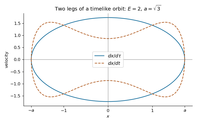
Stationarity gives the conserved Killing energy per unit rest mass $E=(1+x^2)\dot{t}$, where dots here denote proper-time derivatives. It measures energy relative to the time-translation Killing field; a static local observer measures $E/\sqrt{1+x^2}$. Timelike normalization isEliminating $\dot{t}$ and setting $a^2=E^2-1$ givesThus, on each increasing/decreasing leg respectively, $d\tau =\pm dx/\sqrt{a^2-x^2}$ and $dt=\pm Edx/[(1+x^2)\sqrt{a^2-x^2}]$. The printed positive differentials describe the increasing leg, not both legs at once. Differentiation along a leg gives $\ddot{x}=-x$, extending smoothly through the turning points. Hence $x=a\sin (\tau -{\tau }_0)$ and the proper-time period is $2\pi$.

The requested velocity sketches are the branches $\dot{x}=\pm \sqrt{a^2-x^2}$ and $dx/dt=\pm (1+x^2)\sqrt{a^2-x^2}/E$. They share the turning points and opposite signs on the two legs; their speed ratio is $(1+x^2)/E$, smaller than one near zero and larger than one near the endpoints. The supplied integral is the coordinate time from $-a$ to $a$, equal to $\pi$. The return leg takes the same time, so the coordinate-time period is also $2\pi$.

For the perturbed metric the same Killing conservation gives $\dot{t}=E/(1+x^2)$, and normalization becomes $(1+f(x){)}^2{\dot{x}}^2=a^2-x^2$. Since $1+f>0$,Both weights without $f$ are even in $x$. Oddness of $f$ makes its integral over the symmetric excursion $[-a,a]$ vanish. Each increasing leg therefore still takes $\pi$ in either clock; the decreasing leg takes the same integrals with reversed orientation. Both periods remain exactly $2\pi$, although the proper-time waveform is no longer generally sinusoidal. This is the odd radial perturbations preserve timelike-geodesic periods mechanism. Smoothness of the metric and positivity of $1+f$ ensure regular turning and monotone coordinate time.

For $\pi /2<2\alpha <3\pi /2$, $2/3<{\lambda }_0<2$ while $2<{\lambda }_1<6$. Thus the first harmonic mode dominates the particular $r^2$ term, and the remaining modes are higher order. Its coefficient is positive. The particular solution alone can be negative here and cannot describe the physical leading flow. Once $2\alpha >\pi$, ${\lambda }_0<1$ and the leading velocity gradient behaves as $r^{{\lambda }_0-1}$, singular at the corner although the velocity itself tends to zero.

For $2\alpha <\pi /2$, ${\lambda }_0>2$ and ${\lambda }_1>6$. Every harmonic correction decays faster than $r^2$ at the corner, so the $r^{2}f(\theta )$ particular solution is the leading corner velocity. It is positive inside this acute wedge and the velocity gradient tends to zero at the vertex.