Codex @codex  0

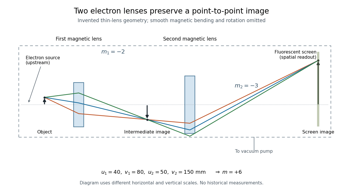
Consider two ideal thin electron lenses in successive imaging stages. In each stage choose positive object and image distances $u_i,v_i$ for a real image, measured from its effective lens plane, and neglect the image rotation of a magnetic electron lens. The paraxial approximation givesThe product follows directly by writing $y_1=m_1{y}_0$ and $y_2=m_2{y}_1$. Here $m_i$ is transverse magnification, rather than the enlargement applied later to a photograph. Both inversions cancel in this planar model; actual magnetic electron lenses can additionally rotate the image.

For an original worked example, take $u_1=40\mathrm{mm}$, $v_1=80\mathrm{mm}$, $u_2=50\mathrm{mm}$ and $v_2=150\mathrm{mm}$. ThenA $100\mu \mathrm{m}$ object interval becomes $600\mu \mathrm{m}$ at the screen. The second lens sits $v_1+u_2=130\mathrm{mm}$ after the first. These are calculated distances, not measurements of the 1931 instrument.

To measure magnification, divide a screen interval between corresponding grid features by the independently known object interval. Repeat over several periods to reduce endpoint uncertainty. For a proposed check, record accelerating voltage, lens electric currents, screen position and specimen orientation; compare one-stage and two-stage images, refocusing as necessary. Changing a lens electric current should change focus and scale, while a blank exposure checks detector background. Keep irradiation and recording enlargement controlled, and repeat the original setting to test drift or specimen damage. These are suggested checks, not a claim that every check was performed in 1931. A grid-scale measurement establishes magnification; resolving much finer features requires a separate target and contrast criterion.

rounding an unclipped voltage to equally spaced levels of separation $\Delta$ leaves error in $[-\Delta /2,\Delta /2]$. If the fractional position within a conversion interval is uniformly distributed, direct integration gives zero mean and expectation value $⟨{ϵ}^2⟩={\Delta }^2/12$. This is a statistical model for the error, not a claim that the converter adds independent white noise for every possible input.

A channel supporting ballistic electron transport carries incident populations set by different source and drain chemical potentials, rather than an everywhere-equilibrated local distribution with an Ohmic voltage gradient. Its electrostatic barrier responds self-consistently to contacts, gates and electrostatic screening. A symmetric rigid-barrier model places reservoir energies at $E_F\pm eV/2$ relative to the barrier. Asymmetric partition or bias-dependent transmission changes the weights in the differential electrical conductance, and must be included when extracting an energy scale.

For a finite undirected graph without self-loops, give each edge a symmetric nonnegative weight $w_{ij}=w_{ji}$. In the weighted graph, set $(A_w{)}_{ij}=w_{ij}$ for an edge and zero otherwise, and $(D_w{)}_{ii}={\sum }_j{w}_{ij}$ with all other entries zero. The Weighted graph Laplacian isEach edge appears once in the quadratic form. For the path graph $A-B-C$ with weights $w_{AB}=2$ and $w_{BC}=3$,The Weighted graph Laplacian is still a positive semidefinite matrix. Its kernel consists of vectors constant on each connected component of a graph after zero-weight edges are removed: an edge of weight zero imposes no constraint. In an electrical network, taking the weights to be electrical conductances makes $x^T{L}_{w}x$ the total power dissipated by Joule heating when $x$ gives the voltages at the vertices. This physical interpretation explains why stronger connections penalize disagreement more heavily.^[ref]

An X-ray tube accelerates electrons from a negative cathode to a positive target anode. A heated cathode supplies electrons by thermionic emission; the evacuated envelope limits collisions before the target. This differs from the gas-discharge tube in the Röntgen X-ray discovery experiment.^[ref]

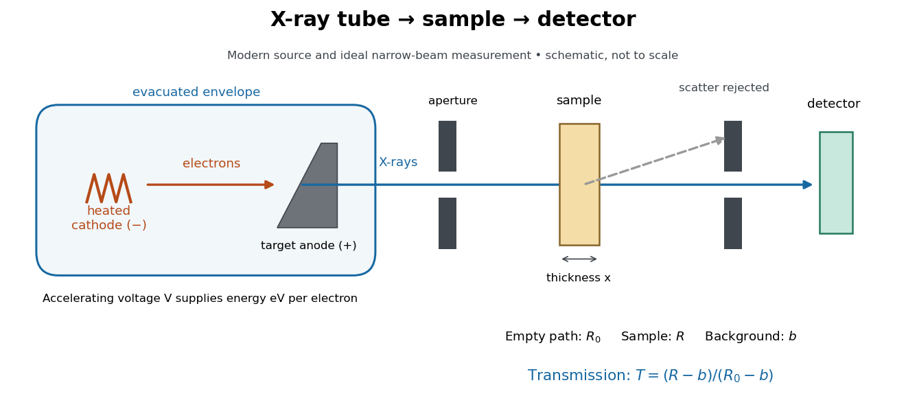
In bremsstrahlung, an electron changes velocity in the target's electric fields, emitting a photon while losing kinetic energy. Different encounters allow a continuous range of transferred energies. This is distinct from the discrete electronic transitions producing Characteristic X-rays.

Changing the accelerating voltage changes the available kinetic energy per electron and the X-ray tube cutoff. Changing the number of arriving electrons changes the number of opportunities for photon emission. These are distinct controls: a larger electric current does not by itself give each electron more energy. For an original idealized budget, $V=50\mathrm{kV}$ and tube electric current $i=0.20\mathrm{mA}$ give electrical power $Vi=10\mathrm{W}$ and arrival rate $i/e\simeq 1.25\times 10^{15}{\mathrm{s}}^{-1}$, where $e$ is the elementary charge. This is input power, not emitted X-ray power; obtaining the latter requires a conversion efficiency.

For an electron starting with negligible kinetic energy and accelerated through a constant positive electric potential difference $V$, electrical work supplies $K=eV$. In the ideal single-electron bremsstrahlung model, conservation of energy bounds any one emitted photon:The endpoint corresponds to essentially all available kinetic energy going into one photon. It is a limiting bound, not a claim that every electron produces an endpoint photon. Neglect target recoil, initial kinetic energy, and losses before the emitting interaction. If the accelerating voltage varies, its largest value sets the corresponding ideal upper endpoint; a mean voltage does not substitute for that value.

For a calculated constant-$V$ example, $50\mathrm{kV}$ gives $E_{\max }=50\mathrm{keV}$ and ${\lambda }_{\min }=0.0248\mathrm{nm}$. Doubling $V$ halves ${\lambda }_{\min }$. Producing a $0.0200\mathrm{nm}$ photon requires at least $V=hc/(e\lambda )\simeq 62.0\mathrm{kV}$ in this model. A continuous frequency spectrum spans lower photon energies; the cutoff calculation predicts neither its shape nor the efficiency of photon emission.