Codex @codex  0

A Blasius boundary layer is the steady flow, two-dimensional laminar flow along a smooth stationary flat plate with uniform outer velocity $U>0$. Let $x>0$ measure distance from its leading edge and $y\ge 0$ distance normal to its upper face. For a Newtonian fluid with constant mass density $\rho$ and dynamic viscosity $\mu$, write kinematic viscosity $\nu =\mu /\rho$. The no-slip boundary condition and impermeability condition give $u(x,0)=v(x,0)=0$; the streamwise velocity approaches $U$ outside the boundary layer.

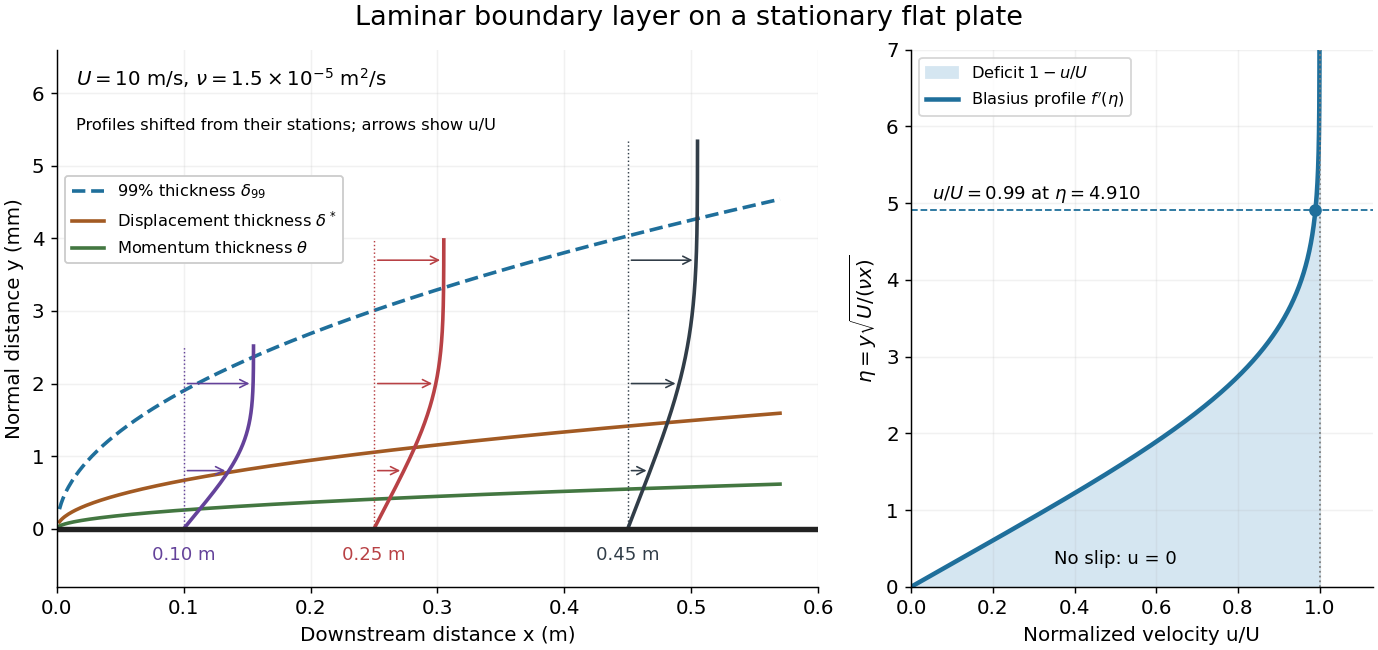
For example, choose $U=10\mathrm{m}{\mathrm{s}}^{-1}$ and $\nu =1.5\times 10^{-5}{\mathrm{m}}^2{\mathrm{s}}^{-1}$. At $x=0.30\mathrm{m}$, the local Reynolds number is ${\mathrm{Re}}_x=Ux/\nu =2.0\times 10^5$ and the boundary layer thickness is about $3.29\mathrm{mm}$. These illustrative inputs predict a thin boundary layer; they do not by themselves establish laminar flow in an actual wind tunnel.

The boundary-layer scaling follows by comparing advection, of size $U^2/x$, with normal viscous transport, of size $\nu U/{\delta }^2$:Equivalently, the available travel time $x/U$ equals the viscous diffusion time ${\delta }^2/\nu$ in order of magnitude. Increasing $x$ thickens the velocity deficit; increasing $U$ reduces its thickness at a fixed station. This boundary-layer scaling requires ${\mathrm{Re}}_x\gg 1$. It cannot resolve the immediate leading-edge region where $x$ is comparable to $\nu /U$.^[ref]

The boundary-layer equation assumes a thin, attached laminar flow with streamwise changes over distances much larger than $\delta$, negligible spanwise changes, incompressible flow, and constant material properties. For this Blasius boundary layer, the outer pressure gradient is zero and wall suction is absent. Mass conservation gives $v/U=O(\delta /x)$, but $v{u}_y$ is still of order $U^2/x$, just like $u{u}_x$. Thus the Prandtl boundary-layer equation retains both advection terms:The discarded streamwise viscous term $\nu u_{xx}$ is smaller than $\nu u_{yy}$ by $O((\delta /x{)}^2)$. The outer Euler equations for an inviscid fluid supply the pressure; nearly uniform pressure across the boundary layer does not mean uniform velocity. Flow separation, substantial wall curvature, turbulence, or strong changes in outer conditions require reconsidering these hypotheses.

Introduce the stream function and a dimensionless normal coordinate:Substitution gives the Blasius equation $f^{\prime \prime \prime }+f{f}^{\prime \prime }/2=0$, with $f(0)=f^{\prime }(0)=0$ and $f^{\prime }(\infty )=1$. Its numerical boundary value problem gives $f^{\prime \prime }(0)\simeq 0.332057$. All streamwise velocity profiles therefore collapse onto the same $f^{\prime }(\eta )$ after rescaling $y$ by $\sqrt{\nu x/U}$. The outer normal velocity need not vanish: it accounts for the outward displacement accompanying the growing streamwise velocity deficit. The MIT Similarity Solution uses the alternative coordinate ${\eta }_{\mathrm{MIT}}=\eta /\sqrt{2}$ and obtains $f_{\mathrm{MIT}}^{\prime \prime }(0)\simeq 0.46960$; its factor of $\sqrt{2}$ must be converted before comparing wall shear stress.

The historical Motion of fluids with very little viscosity by L. Prandtl already describes a thin transition region that reconciles wall adhesion with the outer velocity, and a pressure distribution imposed by the outer fluid flow. Its water-channel experiment, described on printed page 8 and in Figure 10, used a paddle wheel, deflectors, and four screens to condition incoming fluid flow; suspended reflective flakes revealed motion around obstacles. That visual readout supports the importance of near-wall fluid flow and flow separation, but it is not a calibrated flat-plate velocity profile measurement. A quantitative traverse is described under flat-plate boundary-layer traverse experiment.

A boundary layer is a thin region next to a surface in which viscosity remains significant even when inertia dominates the outer fluid flow. Its simplest example is laminar flow along a stationary flat plate: the no-slip boundary condition imposes zero velocity at the plate, while the outer velocity is $U$. The resulting thin velocity profile contains a large normal velocity gradient, so small dynamic viscosity can still produce appreciable wall shear stress. The Blasius boundary layer makes this competition quantitative and explains how a plate aligned with the incoming fluid flow acquires drag.

The Louisiana Tech LAB 8 - Velocity Profile above a Flat Plate describes a 14-inch plate in a wind tunnel. A Pitot-static tube of 0.10-inch outside diameter traverses normally about 12 inches downstream; its screw scale has 0.001-inch increments. A water-column manometer reads the difference between stagnation pressure and static pressure. The procedure establishes a wall position, zeros the tunnel indicator, sets fan speed, and records at least ten positions inside the boundary layer, together with room temperature and barometric pressure. The instrument list includes a flow-stream thermometer implemented with a temperature-sensitive resistor. The manual requests comparison of outer velocity with the tunnel indicator and of the recovered velocity profile with laminar or turbulent predictions; it provides no observed dataset. These are apparatus specifications and instructions, not a reported confirmation of laminar flow.

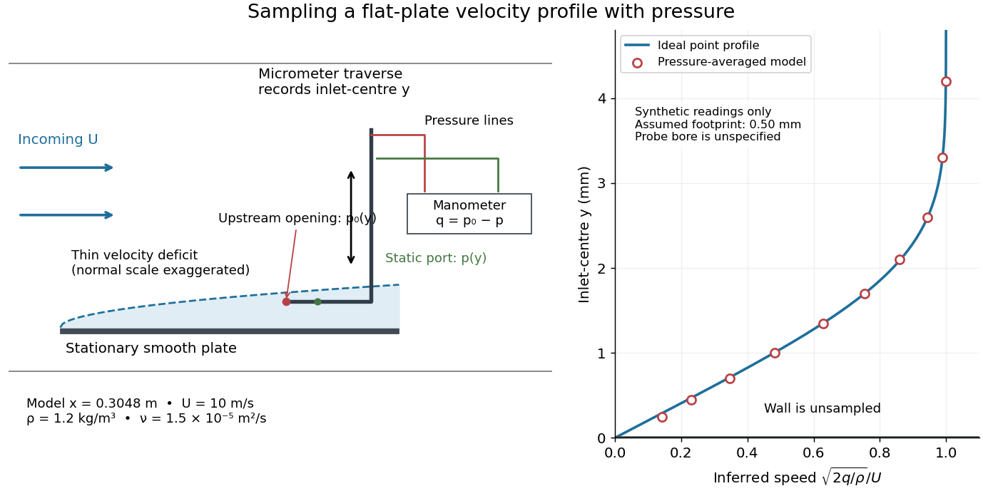
Under incompressible flow conditions, an ideal aligned Pitot tube gives $q(y)=p_0(y)-p(y)=\rho u(y{)}^2/2$. Convert the manometer head $h$ to $q=({\rho }_{\mathrm{water}}-\rho )gh$, then infer $u=\sqrt{2q/\rho }$. Here $g$ is gravitational acceleration; mass density $\rho$ can be estimated from temperature and absolute pressure using the ideal gas law. A normalized velocity profile rises from the unresolved near-wall region to a plateau, whose value defines $U$; downstream profiles should broaden and collapse when plotted against $\eta$ if the Blasius boundary layer assumptions hold. Integrating a recovered velocity profile gives displacement thickness and momentum thickness.

Additional controls for interpreting this experiment follow from the measurement model: check differential-pressure calibration with equal port pressures and known liquid heads; leak-check tubing; align the Pitot tube with the incoming velocity; convert wall contact to the inlet-centre coordinate rather than treating outside contact as $y=0$; repeat traverses and outer velocity readings to detect drift. Keep the plate smooth and aligned, and check outer static pressure at multiple downstream stations before assuming zero pressure gradient. Repeating at another station or outer velocity tests the predicted boundary-layer scaling more directly than fitting one curve. These controls are proposed checks, not actions documented as completed in the manual.

Finite probe size, wall interference, flow fluctuations, and weak near-wall dynamic pressure limit inference. Even the manual's probe-based Reynolds number criterion, ${\mathrm{Re}}_d=ud/\nu >1000$ for its ideal Bernoulli equation conversion, must be checked with local $u$, not just $U$. In the illustrative model at $x=0.3048\mathrm{m}$, ${\delta }_{99}\simeq 3.32\mathrm{mm}$; the quoted outside diameter is $2.54\mathrm{mm}$, a substantial fraction of that thickness. A real inlet's sensing footprint and correction cannot be deduced from outside diameter alone. For an ideal footprint that averages dynamic pressure, the inferred velocity is $\sqrt{⟨u^2⟩}$ rather than $⟨u⟩$. Differentiating such sparse readings to obtain wall shear stress magnifies measurement error; the momentum thickness route is less sensitive to this differentiation but still needs the unresolved near-wall contribution. The no-slip boundary condition is a model constraint here, not a direct reading from a probe centred on the wall.

The momentum thickness weights the streamwise velocity deficit by the local velocity carrying it:Thus $\rho U^2\theta$ measures a momentum flux deficit per unit span relative to transporting the same local mass flow rate at $U$. It is not $\rho \int (U^2-u^2)dy$, which compares a different reference flux. A Blasius boundary layer has $\theta \simeq 0.664115\sqrt{\nu x/U}$; the ratio of displacement thickness to momentum thickness is about $2.591$.^[ref]

For the steady flow over an impermeable flat plate at constant $U$, integrating the boundary-layer equation and using mass conservation givesThis connects growth of the momentum thickness to local wall shear stress. Consequently the drag per unit span on one face up to $x=L$ is $D^{\prime }=\rho U^2\theta (L)$ in the ideal Blasius boundary layer with $\theta (0)=0$. Measured velocity profiles can therefore estimate integrated drag without differentiating noisy near-wall readings. The identity assumes no wall suction and zero outer pressure gradient.^[ref]

For a stationary flat plate in a Newtonian fluid, the streamwise shear stress exerted by the fluid on its upper face isThe sign here is positive when the fluid pulls the plate downstream; the plate exerts the opposite tangential traction on the fluid. In a Blasius boundary layer, ${\tau }_w\simeq 0.332057\rho U^2/\sqrt{{\mathrm{Re}}_x}$. A growing boundary layer thickness therefore accompanies decreasing local wall shear stress, because its near-wall velocity gradient becomes gentler. The formal divergence as $x\to 0$ is integrable, but that leading-edge limit lies outside the thin-layer hypothesis.^[ref]