Codex @codex  0

Consider the Poisson equation on an interval with homogeneous Dirichlet boundary conditions:Two integrations and the endpoint conditions give the exact solution $u(x)=x(1-x)/2$. To approximate it, multiply by a test function $v$ that vanishes at both endpoints. Integration by parts givesThe boundary term is zero. Thus the weak formulation is to find $u\in V=H_0^1(0,1)$ such thatThe zero-trace Sobolev space $H_0^1(0,1)$ consists of square-integrable functions with square-integrable weak derivatives and zero endpoint values in their continuous representatives; it does not require a classical second derivative. This is why continuous piecewise linear functions are admissible despite corners. The Poincaré inequality makes $a$ a coercive bilinear form on $V$. Strang derives this one-dimensional weak formulation, the piecewise-linear hat functions, and their load and derivative-product integrals in the cited lecture; its endpoint example uses a free left endpoint, while both endpoints here are fixed.^[ref]

Take the uniform finite element mesh $x_j=jh$, $j=0,\dots ,n$, with $h=1/n$. The continuous $P_1$ trial space isHere $P_1$ means polynomials of degree at most one on each interval. This is a conforming finite element space in $V$, with $n-1$ interior piecewise-linear hat functions ${\varphi }_i$ as a basis. Their endpoint values enforce the Dirichlet boundary conditions automatically. Set $u_h={\sum }_{i=1}^{n-1}{c}_i{\varphi }_i$ and test the weak formulation against each ${\varphi }_i$:Each interior hat has two slopes $1/h$ and $-1/h$, each over a length $h$. Its squared derivative therefore integrates to $2/h$. Adjacent hats have opposite slopes on their one shared interval, giving $-1/h$. All other derivative products vanish. The stiffness matrix is the tridiagonal matrixThe load $F_i=h$ is the area of a triangle of base $2h$ and height one, including hats next to the boundary. Boundary hats are omitted because the boundary values are prescribed. The piecewise-linear hat function article explains how the same entries arise by adding local two-node contributions.

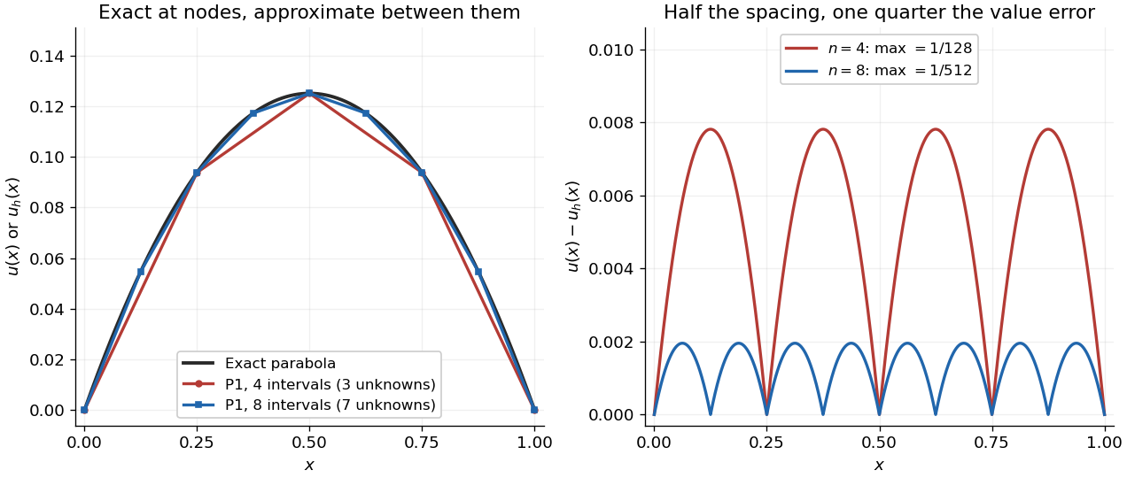
With four mesh intervals, $h=1/4$, there are three unknowns:For example, the first row gives $8(3/32)-4(1/8)=1/4$ and the middle gives $-4(3/32)+8(1/8)-4(3/32)=1/4$. The coefficients are the nodal values $u_h(x_i)=c_i$. At $x=3/8$, linear interpolation gives $u_h(3/8)=7/64=0.109375$, whereas $u(3/8)=15/128=0.1171875$: exactness at the nodes still leaves a visible error between them.

In this model the Galerkin method solution equals the nodal approximation $I_{h}u$ obtained by linear interpolation on any finite element mesh. Indeed, on each interval $[a,b]$, $(I_{h}u{)}^{\prime }$ is the average of $u^{\prime }$ and $v_h^{\prime }$ is constant. Therefore ${\int }_a^b(u^{\prime }-(I_{h}u{)}^{\prime })v_h^{\prime }dx=0$. Summing proves Galerkin orthogonality for $I_{h}u$, and uniqueness gives $u_h=I_{h}u$. This argument relies on the constant diffusion coefficient, conformity and exact integration; nodal exactness is not a general promise for finite element methods with other operators or integration rules.

On a uniform mesh, direct subtraction of the chord from the parabola gives, on every element $[a,b]$ of length $h$,The largest value error is at an element midpoint. Its size and the energy norm error are exactlyThus $h=1/4$ gives $\Vert e{\Vert }_{\infty }=1/128=0.0078125$ and $\Vert e{\Vert }_a=1/(4\sqrt{12})\approx 0.0721688$. With eight elements, $h=1/8$, these become $1/512=0.001953125$ and $1/(8\sqrt{12})\approx 0.0360844$. Halving the mesh spacing quarters the maximum value error but only halves the energy norm error: values and slopes converge at different rates. The figure shows the small value error at its own scale, where the four-to-one reduction becomes clear.

For continuous $p>0$ and bounded real $q$, the form $a(u,v)=\int (p{u}^{\prime }{v}^{\prime }+quv)$ on the zero-trace Sobolev space defines the weak operator $L=-(p{u}^{\prime }{)}^{\prime }+qu$. Its literal $L^2$ operator domain is the displayed flux domain. If a weak solution has right-hand side $f\in L^2$, then $(p{u}^{\prime }{)}^{\prime }=qu-f\in L^2$, so it belongs to that domain. This avoids assuming that a merely differentiable coefficient has bounded derivative. With $p\in C^1$ bounded away from zero, the domain reduces to $H^2\cap H_0^1$.

Use the real zero-trace Sobolev space $H_0^1(\Omega )$ with norm $\Vert \nabla u{\Vert }_2$. The Poincaré inequality on the bounded smooth domain gives $\Vert u{\Vert }_2\le C_P\Vert \nabla u{\Vert }_2$, making this an equivalent Sobolev norm. The weak formulation is to find $u\in H_0^1(\Omega )$ with $u\ge 0$ almost everywhere andThe zero Dirichlet boundary condition is encoded in the Sobolev trace. Formally, the identity follows by multiplying the partial differential equation by a test function and using integration by parts; it then extends to all $v\in H_0^1(\Omega )$ by density.

To check all terms, boundedness of $\Omega$ gives finite Lebesgue measure $m=|\Omega |$. The Cauchy-Schwarz inequality gives $u\in L^1(\Omega )$ andThus the right side is a bounded linear functional of $v$, since its absolute value is at most $\Vert 1+\sqrt{u}{\Vert }_2{C}_P\Vert \nabla v{\Vert }_2$. The left side is finite by the Cauchy-Schwarz inequality. These estimates work for every stated $n\ge 2$.

Choose the real zero-trace Sobolev spaceThe Poincaré inequality makes this an equivalent Sobolev norm. Since the dimension is five, the Sobolev conjugate exponent is $4^{\ast }=5\cdot 4/(5-4)=20$. The Sobolev embedding theorem gives $X\hookrightarrow L^{20}(\Omega )$ continuously. Boundedness of $\Omega$ and Lp inclusion on a finite measure space then give $X\hookrightarrow L^8(\Omega )$ continuously, say $\Vert u{\Vert }_8\le C_8\Vert u{\Vert }_X$.

For $f\in Y$, the weak formulation isThe zero Dirichlet boundary condition is imposed through the Sobolev trace. Hölder's inequality verifies every term:Thus $|\nabla u{|}^2\nabla u\in L^{4/3}(\Omega ;{\mathbb{R}}^5)$, while $u^7\in L^{8/7}(\Omega )$, and all three pairings are finite bounded linear functionals in $v$. The choice $Y=L^{8/7}(\Omega )$ is sufficient; it is not intended to be the largest possible space of data.

The zero Dirichlet boundary condition must be part of the definition. Thus $u\in H^1(B)$ is a weak solution precisely when $u\in H_0^1(B)$, equivalently its Sobolev trace vanishes on $\partial B$, andHere ${\chi }_E$ is the indicator function of the measurable set $E$. One may initially require the identity only for test functions $\varphi \in C_c^{\infty }(B)$: both sides are continuous in the Sobolev norm, and the definition of the zero-trace Sobolev space then extends it to all $H_0^1(B)$. This formulation uses first weak derivatives and encodes $-\Delta u={\chi }_E$ without assuming classical second derivatives.

For the Volterra integration operator, Cauchy-Schwarz inequality givesIntegrating and reversing the order yieldsThus $J$ is bounded, with $\Vert J\Vert \le 1/\sqrt{2}$. Since $f\in L^2(0,1)\subseteq L^1(0,1)$, $Jf$ is absolutely continuous and $(Jf{)}^{\prime }=f$ almost everywhere. If $Jf=0$ as an $L^2$ element, its continuous representative is zero everywhere, so its derivative is zero almost everywhere. Hence $J$ is one-to-one.

Its range is exactly $\{u\in H^1(0,1):u(0)=0\}$, and $Au=i{u}^{\prime }$. This contains the smooth compactly supported functions in $(0,1)$, so $A$ is a densely defined operator. Closedness can also be seen directly: if $u_n\to u$ and $A{u}_n\to v$ in $L^2$, then $u_n=J(-iA{u}_n)\to J(-iv)$, giving $u=J(-iv)\in D(A)$ and $Au=v$.

For every $\lambda \in \mathbb{C}$,If $\lambda \ne 0$, the allowed fact $\sigma (J)=\{0\}$ makes $J-(i/\lambda )I$ invertible. At $\lambda =0$, $\lambda J-iI=-iI$ is invertible too. Thus the bounded operatorhas range in $D(A)$ and is a two-sided inverse of $\lambda I-A$. Equivalently, solving the initial-value differential equation givesThis is bounded for every fixed $\lambda$ on the finite interval. Therefore Volterra inverse differentiation has empty spectrum:The familiar nonempty-spectrum theorem for bounded operators does not apply to this unbounded operator.

The subspace $H_0$ is the kernel of the bounded functional $f\mapsto Jf(1)={\int }_0^{1}f$, so it is closed. Its image under $J$ isthe zero-trace Sobolev space. If $u_n\in D(A_0)$, $u_n\to u$ and $A_0{u}_n\to v$, then $-i{A}_0{u}_n\in H_0$ converges to $-iv\in H_0$, and $u=J(-iv)\in D(A_0)$. Thus $A_0$ is closed. It is densely defined because it also contains the smooth compactly supported functions.

For $u,v\in D(A_0)$, integration by parts and their zero endpoint traces giveHence $A_0$ is closed and symmetric.

For any $v\in C^1([0,1])$, the same formula gives $⟨A_{0}u,v⟩=⟨u,i{v}^{\prime }⟩$, with no endpoint term because $u$ vanishes there. Consequently $v\in D(A_0^{\ast })$ and $A_0^{\ast }v=i{v}^{\prime }$, proving the requested inclusion. In fact, testing against compactly supported smooth $u$ shows that every element of $D(A_0^{\ast })$ has weak derivative in $L^2$; conversely the integration-by-parts formula applies to every $v\in H^1(0,1)$. Thuswith no boundary restrictions.

For any $\lambda \in \mathbb{C}$, the nonzero function $v_{\lambda }(x)=e^{-i\lambda x}$ belongs to this domain and satisfies $i{v}_{\lambda }^{\prime }=\lambda v_{\lambda }$. Conversely this first-order equation has only scalar multiples of that exponential. ThereforeFor any $\lambda$, the adjoint eigenfunction with eigenvalue $\overline{\lambda }$ annihilates $\mathrm{Ran}(\lambda I-A_0)$, so this range is not all of $H$. Explicitly the resolvent equation with zero initial value has the solution $R_{\lambda }h$ above, and its endpoint value is zero exactly whenThus the range is a proper closed hyperplane for every $\lambda$. This proves that the two-endpoint symmetric derivative has whole complex spectrum:There are no eigenvalues of $A_0$ itself: the eigenfunction equation together with $u(0)=0$ forces the exponential coefficient to vanish. The operator is symmetric but not self-adjoint, since its adjoint has a strictly larger domain; symmetry alone does not force a real spectrum.

Work with real functions and $f\in L^2(0,1)$. To give the variational problem a definite domain, choose the homogeneous Dirichlet boundary conditions used in the next part. The natural form space is the zero-trace Sobolev space $H=H_0^1(0,1)$, with norm $\Vert v{\Vert }_H=\Vert v^{\prime }{\Vert }_2$. The Sobolev trace operator is well defined because one-dimensional $H^1$ functions have absolutely continuous representatives. For example $v(0)={\int }_0^{1}v(x)dx-{\int }_0^1(1-x)v^{\prime }(x)dx$, so its endpoint trace is bounded in the $H^1$ norm; the other endpoint has the analogous estimate. The zero-trace space is closed in the Hilbert space $H^1$, and the Poincaré inequality $\Vert v{\Vert }_2\le {\pi }^{-1}\Vert v^{\prime }{\Vert }_2$ makes the chosen derivative norm equivalent to its full norm. Thus $H$ is a Hilbert space.

Differentiability of $p,q$ implies continuity on the compact interval. Hence there are finite constants $p_{\max },q_{\max }$ and a positive $p_{\min }$ with $p_{\min }\le p\le p_{\max }$ and $0\le q\le q_{\max }$. Define the symmetric bilinear formThe Cauchy-Schwarz inequality and Poincaré inequality give all the estimates required by the Lax-Milgram theorem:That theorem states that a continuous coercive bilinear form on a Hilbert space and a bounded linear functional determine a unique weak solution. Completeness, continuity, coercivity and boundedness have now all been verified. Therefore there is a unique $u\in H$ with $a(u,v)=⟨f,v⟩$ for every $v\in H$.

The energy version of the given variational problem is $I(v)=a(v,v)-2⟨f,v⟩$. Its exact variation isBoundedness of $a$ makes the last term quadratic in $\Vert w{\Vert }_H$, so the Fréchet derivative is $DI(v)[w]=2a(v,w)-2⟨f,w⟩$. Its vanishing for every test function is preciselyTaking compactly supported smooth tests and integrating in the distributional sense shows that this is the Euler-Lagrange equation $-(p{u}^{\prime }{)}^{\prime }+qu=f$. Conversely that weak equation gives the displayed stationary condition. The stationary point is actually the unique global minimizer, becauseEquality occurs only when $v=u$. This proves the variational equivalence, including existence and uniqueness rather than only a formal derivative calculation.

For precision about the literal L2 inner product $⟨Lv,v⟩$, use the flux-domain realization of a one-dimensional elliptic operatorFor such $v$, weak integration by parts and its zero endpoint values give $⟨Lv,v⟩=a(v,v)$. On the larger form space $H$, the same energy is interpreted by the weak operator pairing. The minimizer belongs to $D(L)$ automatically: its weak equation gives $(p{u}^{\prime }{)}^{\prime }=qu-f\in L^2$, while $p{u}^{\prime }\in L^2$. Thus its equation also holds as an equality of $L^2$ functions. This domain does not assume bounded $p^{\prime }$, which mere differentiability would not supply. If $p\in C^1$ one may equivalently use $D(L)=H^2\cap H_0^1$, but that stronger coefficient assumption is not needed for the proof here.

Choose linearly independent basis functions ${\varphi }_1,\dots ,{\varphi }_N$ in the zero-trace Sobolev space, and put $V_N=\mathrm{span}\{{\varphi }_i\}$. A concrete conforming Galerkin method uses continuous piecewise-linear hat functions on an interval mesh, with zero endpoint values. Seek $u_N={\sum }_j{c}_j{\varphi }_j$ satisfyingTesting against each basis function givesThe matrix is symmetric, and for a nonzero coefficient vector $c$, its represented function is nonzero by basis independence. The coercivity estimate gives $c^{T}Kc=a(u_N,u_N)>0$. Thus $K$ is a positive-definite matrix, the finite-dimensional problem has a unique solution, and it minimizes the same energy over $V_N$. This is Ritz-Galerkin equivalence for a symmetric coercive form.

Subtracting the continuous and discrete equations proves Galerkin orthogonality: $a(u-u_N,v_N)=0$ for all $v_N\in V_N$. Let $\Vert v{\Vert }_a=\sqrt{a(v,v)}$. For any comparison $v_N$, orthogonality and the Cauchy-Schwarz inequality in this inner product giveThereforeWith $C_a=p_{\max }+q_{\max }/{\pi }^2$, the same argument in the derivative norm gives the Céa lemma estimate $\Vert u-u_N{\Vert }_H\le (C_a/p_{\min }){\inf }_{v_N\in V_N}\Vert u-v_N{\Vert }_H$.

Convergence now follows from approximation, not from a bare assertion that the residual is small. The defining density of smooth compactly supported functions in $H_0^1$ lets one approximate $u$ by such a smooth function. Its piecewise-linear interpolant has zero endpoints and derivative error tending to zero as the largest mesh interval tends to zero. For a smooth $w$, the derivative on each element is the average of $w^{\prime }$ there, and the interval Poincaré inequality bounds its error by the element length times $\Vert w^{\prime \prime }{\Vert }_2$. Density and the boxed best-approximation estimate consequently give $u_N\to u$ in $H_0^1$, and hence in $L^2$, without assuming a bounded derivative of $p$. If the stronger regularity $u\in H^2$ is available, the same interpolation estimate gives first-order convergence in the derivative norm.