Hölder's inequality controls a product using separate information about its two factors. If one factor is large on part of a domain, the other factor's complementary Lp norm limits how much their product can accumulate there. The same statement bounds finite sums, integrals and expected values; no independence is required in the probabilistic version.
Let be conjugate exponents, meaningOn a measure space, if and , then andHere the Lp norms are finite; at exponent the norm uses the essential supremum. For a finite vector, integration with counting measure givesThe first step is the triangle inequality; the second is Hölder's inequality.[ref]
For finite vectors, the endpoint case , is : bound every by its maximum, then sum the . Swapping the factors gives the other endpoint. The choice gives the Cauchy-Schwarz inequality.
The conjugate exponent of is , so . The endpoint conventions pair with and with . Examples are , and . The exponents themselves need not add to one; their reciprocals do.
Take , , and vectors and . Their coordinate products are , soTheir Lp norms give the larger boundThus cancellation explains , and Hölder's inequality explains the remaining gap between and the norm product. Small signed sums need not imply small individual coordinate products.
Now keep and choose . The coordinate products are , with no cancellation, andThe matching powers are , namely .
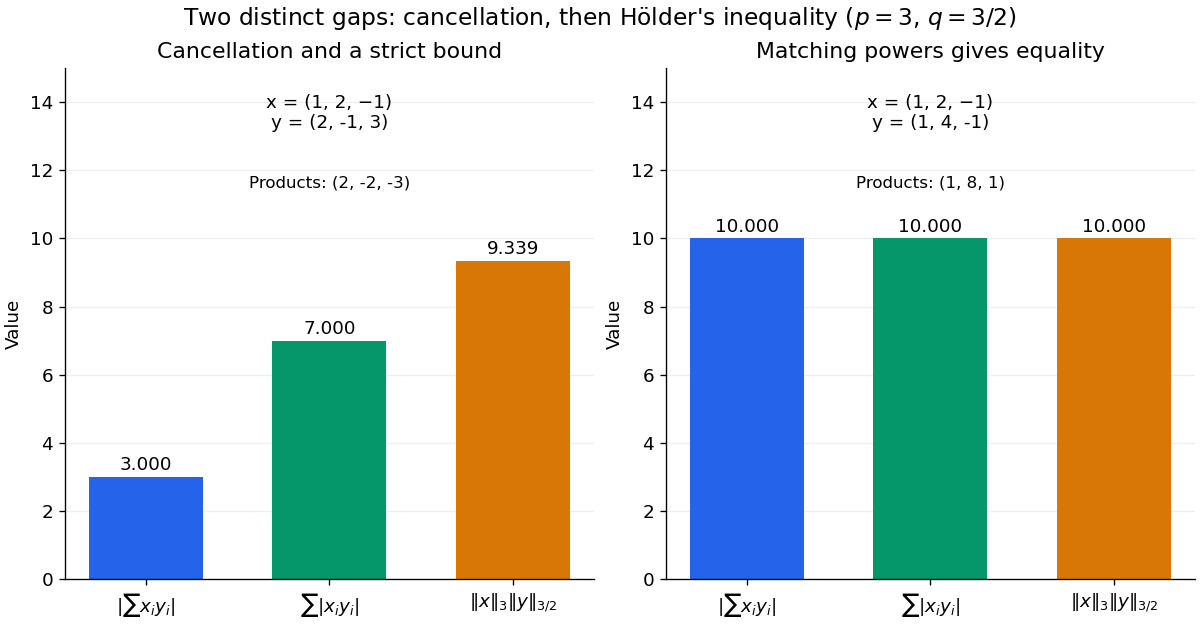
Cancellation and Hölder's inequality account for two different gaps
. Two original finite-vector calculations with , . The first pair has signed sum , absolute-product sum and norm-product bound approximately . The second pair attains equality at . The diagrams show calculated values, with no simulated data. Details.For and nonzero factors in their respective Lp spaces, equality in the product-integral bound holds precisely whenIn other words, the normalized powers match. Zero factors give the trivial equality separately. For real vectors, equality for the signed finite sum also needs the nonzero coordinate products to have a common sign; otherwise the preceding triangle inequality loses information.
For and on , with , ,Changing only to gives , and both sides become . The factors need not be equal: their conjugate powers are what must agree after normalization.
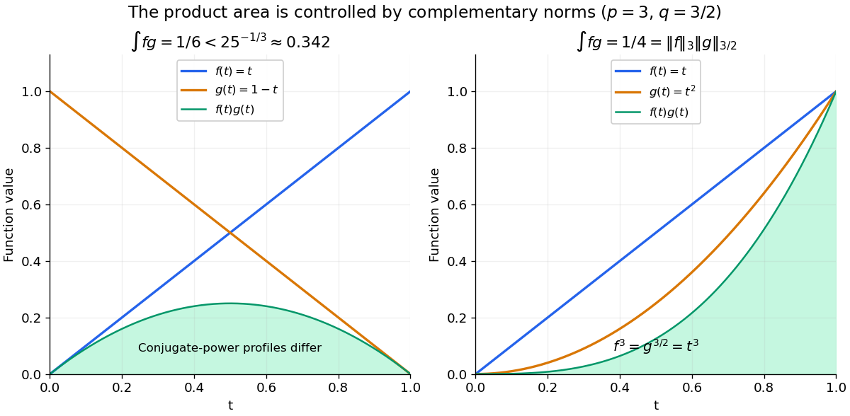
The proof outline makes the equality condition natural. Normalize and . The Young inequality gives ; integration yields . Equality requires almost everywhere. The endpoint proof uses the essential supremum directly, so it does not need division by at .
On a probability space, the same inequality readsIf the displayed moments are finite, the product is an integrable random variable. The random variables can be dependent: the estimate controls their possible overlap without assuming a factorization of the expected value. This is useful when a calculation needs the product to be integrable but the joint probability distribution is complicated.
Otto Hölder's 1889 paper begins with a weighted-mean inequality for a function with increasing derivative. In current terminology, its opening statement is a weighted form of Jensen's inequality: applying a convex function after taking a weighted mean gives a lower bound for the weighted mean of its values. This connects product estimates to the geometry of convex functions, rather than treating them as isolated formulas.[ref]
Ueber einen Mittelwerthssatz by Otto Hölder. Otto Hölder, Ueber einen Mittelwerthssatz (1889), §§1–2, printed pp. 38–39: weighted means and increasing derivative


