How to use an Oxford Nanopore MinION to extract DNA from river water and determine which bacteria live in it PCR by  Ciro Santilli 40 Updated 2025-07-16
Ciro Santilli 40 Updated 2025-07-16More generic PCR information at: Section "Polymerase chain reaction".
Because it is considered the less interesting step, and because it takes quite some time, this step was done by the event organizers between the two event days, so participants did not get to take many photos.
PCR protocols are very standard it seems, all that biologists need to know to reproduce is the time and temperature of each step.
This process used a Marshal Scientific MJ Research PTC-200 Thermal Cycler:

We added PCR primers for regions that surround the 16S DNA. The primers are just bought from a vendor, and we used well known regions are called 27F and 1492R. Here is a paper that analyzes other choices: academic.oup.com/femsle/article/221/2/299/630719 (archive) "Evaluation of primers and PCR conditions for the analysis of 16S rRNA genes from a natural environment" by Yuichi Hongoh, Hiroe Yuzawa, Moriya Ohkuma, Toshiaki Kudo (2003)
One cool thing about the PCR is that we can also add a known barcode at the end of each primer as shown at Code 1. "PCR diagram".
This means that we bought a few different versions of our 27F/1492R primers, each with a different small DNA tag attached directly to them in addition to the matching sequence.
This way, we were able to:
- use a different barcode for samples collected from different locations. This means we
- did PCR separately for each one of them
- for each PCR run, used a different set of primers, each with a different tag
- the primer is still able to attach, and then the tag just gets amplified with the rest of everything!
- sequence them all in one go
- then just from the sequencing output the barcode to determine where each sequence came from!
Input: Bacterial DNA (a little bit)
... --- 27S --- 16S --- 1492R --- ...

|||
|||
vvv

Output: PCR output (a lot of)
Barcode --- 27S --- 16S --- 1492R
Code 1.
PCR diagram
. Finally, after purification, we used the Qiagen QIAquick PCR Purification Kit protocol to purify the generated from unwanted PCR byproducts.
How to use an Oxford Nanopore MinION to extract DNA from river water and determine which bacteria live in it PCR verification with gel electrophoresis by Ciro Santilli 40 Updated 2025-07-16
Ciro Santilli 40 Updated 2025-07-16For this reason, it is wise to verify that certain steps are correct whenever possible.
Gel electrophoresis separates molecules by their charge-to-mass ratio. It is one of those ultra common lab procedures!
Since we know that we amplified the 16S regions which we know the rough size of (there might be a bit of variability across species, but not that much), we were expecting to see a big band at that size.
And that is exactly what we saw!
First we had to prepare the gel, put the gel comb, and pipette the samples into wells present in the gel:


To see the DNA, we added ethidium bromide to the samples, which is a substance that that both binds to DNA and is fluorescent.
Because it interacts heavily with DNA, ethidium bromide is a mutagen, and the biology people sure did treat the dedicated electrophoresis bench area with respect! Figure 4. "Gel electrophoresis dedicated bench area to prevent ethidium bromide contamination.".


Gel electrophoresis dedicated waste bin for centrifuge tubes and pipette tips contaminated with ethidium bromide.
Source. The UV transilluminator we used to shoot UV light into the gel was the Fisher Scientific UVP LM-26E Benchtop 2UV Transilluminator. The fluorescent substance then emitted a light we can see.
As barely seen at Figure 8. "Fischer Scientific UVP LM-26E Benchtop 2UV Transilluminator illuminated gel." due to bad photo quality due to lack of light, there is one strong green line, which compared to the ladder matches our expected 16S length. What we saw it with the naked eyes was very clear however.
How to use an Oxford Nanopore MinION to extract DNA from river water and determine which bacteria live in it Sequencing by Ciro Santilli 40 Updated 2025-07-16
Ciro Santilli 40 Updated 2025-07-16 How to use an Oxford Nanopore MinION to extract DNA from river water and determine which bacteria live in it Using the Oxford Nanopore by Ciro Santilli 40 Updated 2025-07-16
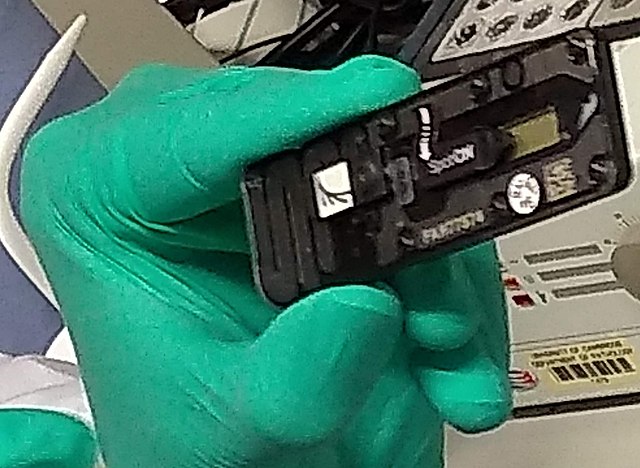
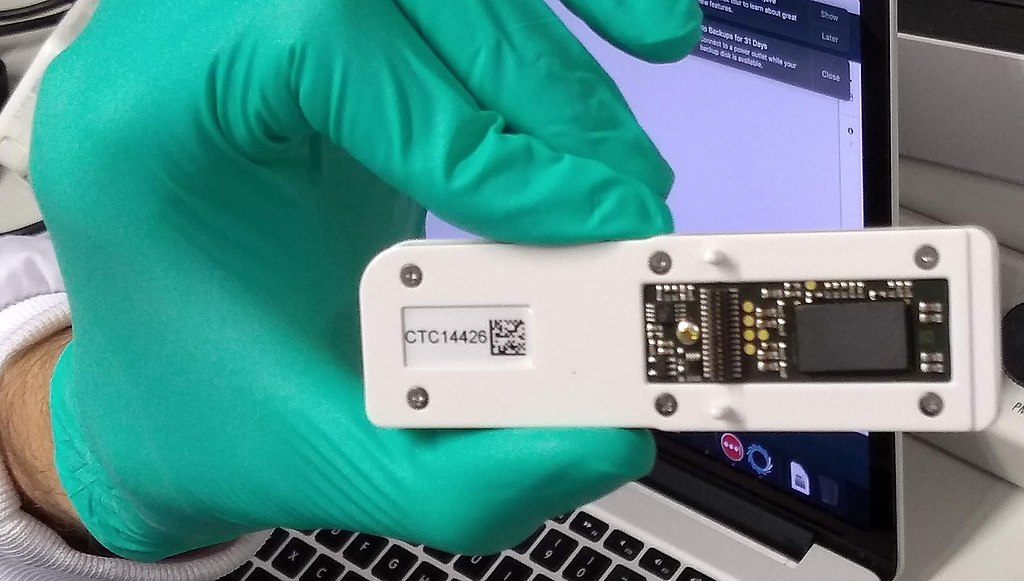
Ciro Santilli 40 Updated 2025-07-16With all this ready, we opened the Nanopore flow cell, which is the 500 dollar consumable piece that goes in the sequencer.
We then had to pipette the final golden Eppendorf into the flow cell. My anxiety levels were going through the roof: Figure 4. "Oxford nanopore MinION flow cell pipette loading.".


At this point bio people start telling lab horror stories of expensive solutions being spilled and people having to recover them from fridge walls, or of how people threw away golden Eppendorfs and had to pick them out of trash bins with hundreds of others looking exactly the same etc. (but also how some discoveries were made like this). This reminded Ciro of: youtu.be/89UNPdNtOoE?t=919 Alfred Maddock's plutonium spill horror story.
Luckily this time, it worked out!
As can be seen from Video 1. "Oxford Nanopore MinION software channels pannel on Mac." the software tells us which pores are still working.
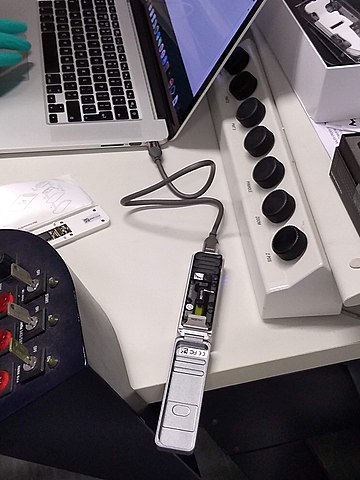
Pores go bad sooner or later randomly, until there are none left, at which point we can stop the process and throw the flow cell away.
48 hours was expected to be a reasonable time until all pores went bad, and so we called it a day, and waited for an email from the PuntSeq team telling us how things went.
We reached a yield of 16 billion base pairs out of the 30Gbp nominal maximum, which the bio people said was not bad.
How to use an Oxford Nanopore MinION to extract DNA from river water and determine which bacteria live in it Qiagen DNeasy PowerWater Kit by Ciro Santilli 40 Updated 2025-07-16
Ciro Santilli 40 Updated 2025-07-16www.qiagen.com/gb/products/discovery-and-translational-research/dna-rna-purification/dna-purification/microbial-dna/dneasy-powerwater-kit (archive) Here is its documentation: www.qiagen.com/gb/resources/download.aspx?id=bb731482-874b-4241-8cf4-c15054e3a4bf&lang=en (archive).

How to use an Oxford Nanopore MinION to extract DNA from river water and determine which bacteria live in it Qiagen QIAquick PCR Purification Kit by Ciro Santilli 40 Updated 2025-07-16
Ciro Santilli 40 Updated 2025-07-16www.qiagen.com/us/products/discovery-translational-research/dna-rn-a-purification/dna-purification/dna-clean-up/qiaquick-pcr-purification-kit/#orderinginformation (archive)
Manual archive: web.archive.org/web/20190911100243/https://www.qiagen.com/us/resources/download.aspx?id=e0fab087-ea52-4c16-b79f-c224bf760c39&lang=en
Removes PCR byproducts from purified DNA.
Microwave only found applications into the 1940s and 1950s, much later than radio, because good enough sources were harder to develop.
One notable development was the cavity magnetron in 1940, which was the basis for the original radar systems of World War II.
Pinned article: Introduction to the OurBigBook Project
Welcome to the OurBigBook Project! Our goal is to create the perfect publishing platform for STEM subjects, and get university-level students to write the best free STEM tutorials ever.
Everyone is welcome to create an account and play with the site: ourbigbook.com/go/register. We belive that students themselves can write amazing tutorials, but teachers are welcome too. You can write about anything you want, it doesn't have to be STEM or even educational. Silly test content is very welcome and you won't be penalized in any way. Just keep it legal!
Intro to OurBigBook
. Source. We have two killer features:
- topics: topics group articles by different users with the same title, e.g. here is the topic for the "Fundamental Theorem of Calculus" ourbigbook.com/go/topic/fundamental-theorem-of-calculusArticles of different users are sorted by upvote within each article page. This feature is a bit like:
- a Wikipedia where each user can have their own version of each article
- a Q&A website like Stack Overflow, where multiple people can give their views on a given topic, and the best ones are sorted by upvote. Except you don't need to wait for someone to ask first, and any topic goes, no matter how narrow or broad
This feature makes it possible for readers to find better explanations of any topic created by other writers. And it allows writers to create an explanation in a place that readers might actually find it.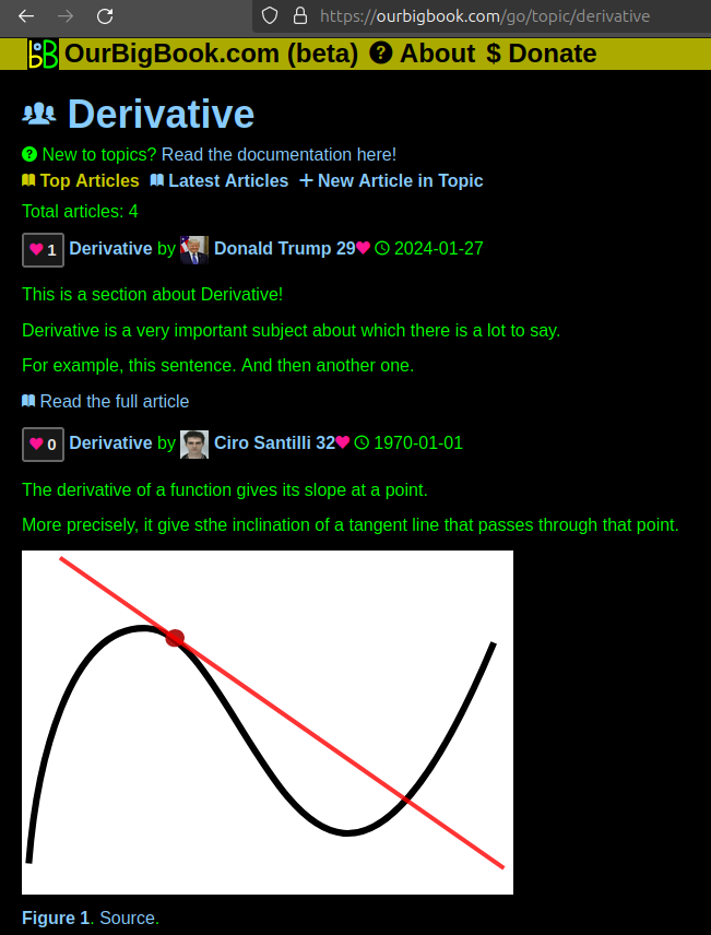
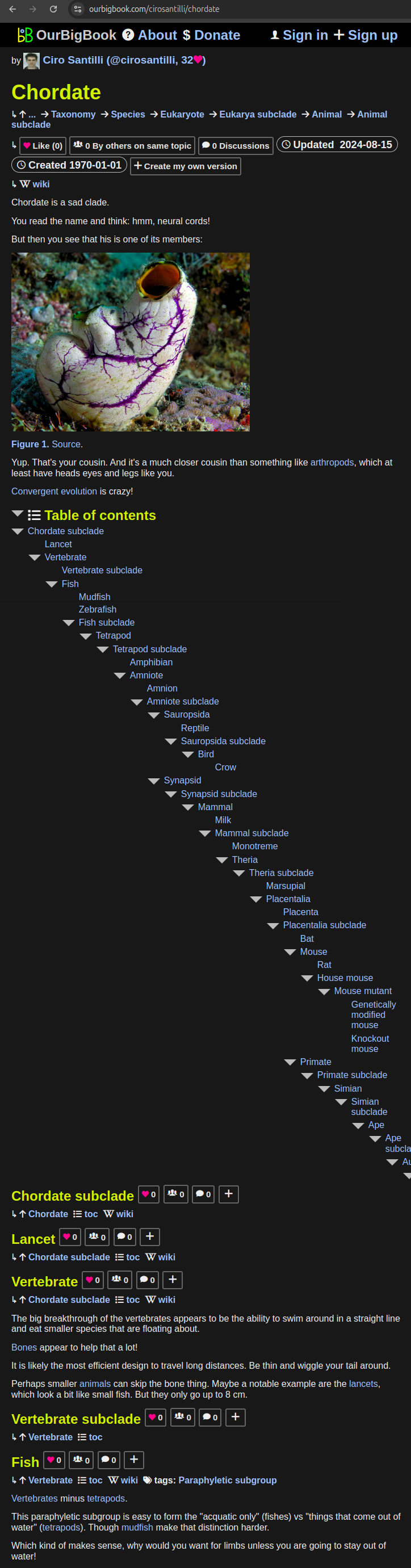
Figure 1. Screenshot of the "Derivative" topic page. View it live at: ourbigbook.com/go/topic/derivativeVideo 2. OurBigBook Web topics demo. Source. - local editing: you can store all your personal knowledge base content locally in a plaintext markup format that can be edited locally and published either:This way you can be sure that even if OurBigBook.com were to go down one day (which we have no plans to do as it is quite cheap to host!), your content will still be perfectly readable as a static site.
- to OurBigBook.com to get awesome multi-user features like topics and likes
- as HTML files to a static website, which you can host yourself for free on many external providers like GitHub Pages, and remain in full control
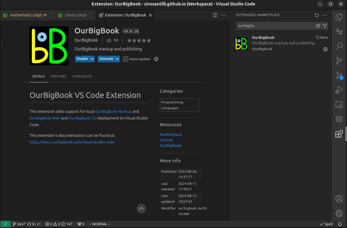
Figure 3. Visual Studio Code extension installation.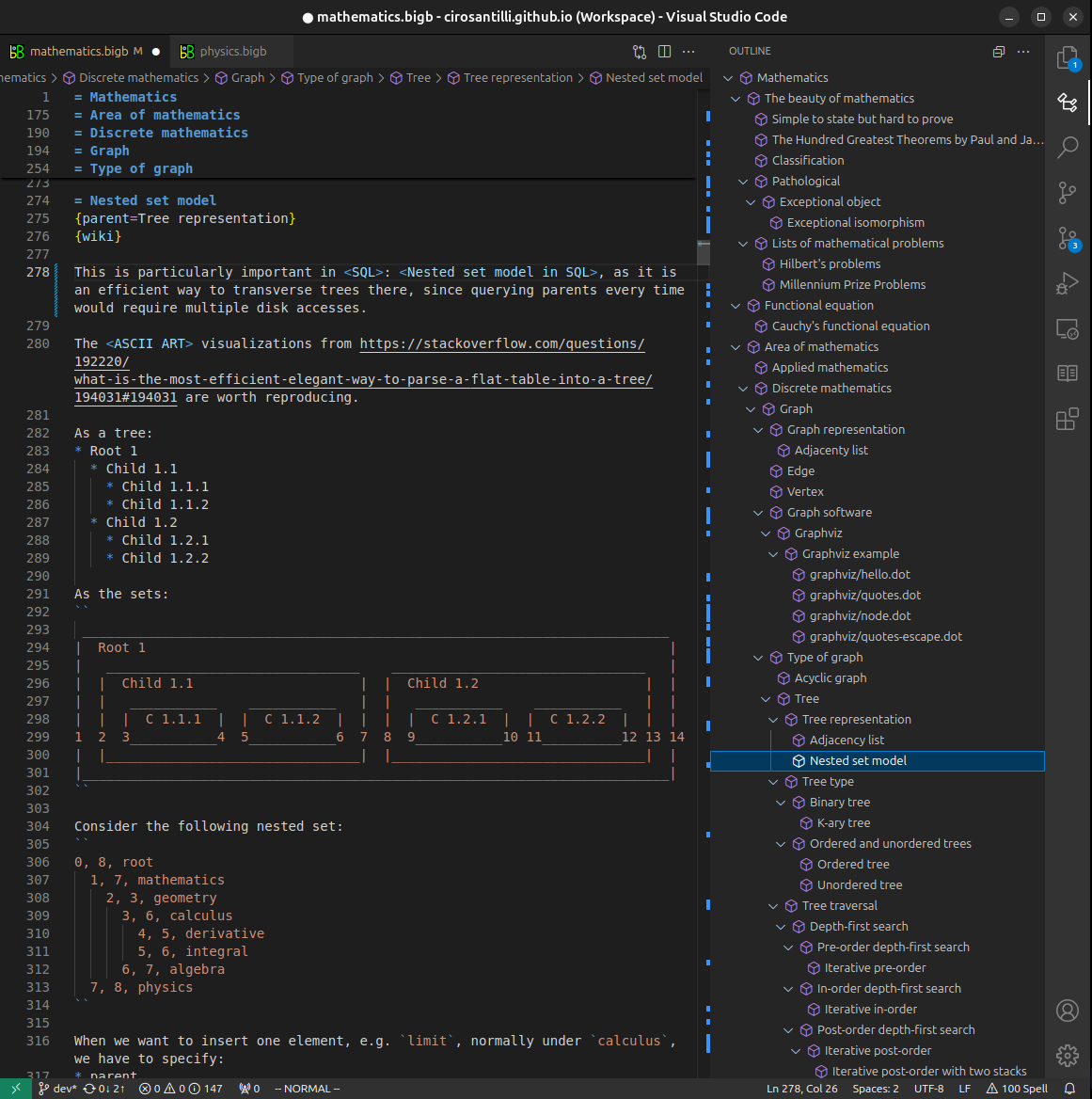
Figure 4. Visual Studio Code extension tree navigation.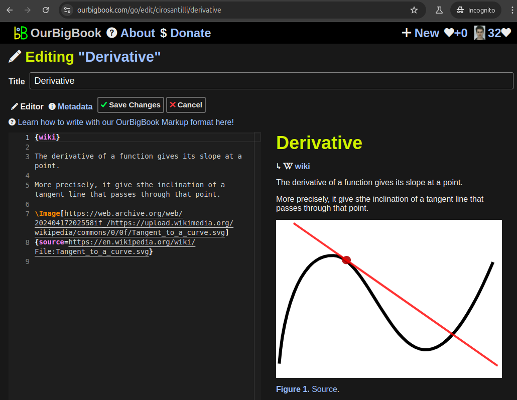
Figure 5. Web editor. You can also edit articles on the Web editor without installing anything locally.Video 3. Edit locally and publish demo. Source. This shows editing OurBigBook Markup and publishing it using the Visual Studio Code extension.Video 4. OurBigBook Visual Studio Code extension editing and navigation demo. Source. 
- Infinitely deep tables of contents:

All our software is open source and hosted at: github.com/ourbigbook/ourbigbook
Further documentation can be found at: docs.ourbigbook.com
Feel free to reach our to us for any help or suggestions: docs.ourbigbook.com/#contact