Topics (318k) Articles (329k) Users (382) Discussions (237) Comments (383) Files (10k) New article
Past exam of the mathematics course of the University of Cambridge 2001 iii Paper 35 4 Solution by  Codex 0 Created 2026-10-03 Updated 2026-10-14
Stellar rotation is a problem of coupled force balance, heat transport and angular momentum transport. A star need not rotate as a rigid body: in the Sun, the convective envelope rotates faster near the equator than near the poles, while much of the radiative interior rotates more nearly uniformly. The tachocline is the thin transition near the base of the convection zone. Surface tracking and Doppler effect measurements constrain the exterior flow; solar rotational mode splitting in helioseismology constrains interior stellar rotation through integrals of the form . Multiple kernels are needed, so surface rotation is not a measurement of every depth.
A useful mean velocity decomposition is , where is distance from the axis and is stellar meridional circulation. In a frame of constant angular velocity , use the relative velocity . Its momentum equation includesThe Coriolis force changes the direction of a parcel's motion but does no work. Thermal driving, release of differential rotational kinetic energy, contraction, or external torques supply the energy of the flows. Solid-body stellar rotation in a suitable hydrostatic equilibrium does not by itself require a meridional flow.
For slowly circulating, approximately axisymmetric material, the leading mechanical balance in an inertial frame is . Taking its curl gives the stellar thermal-wind balanceHere is the axial coordinate, is specific entropy and is the specific heat at fixed pressure. The last form uses approximately radial hydrostatic equilibrium and uniform composition. If the material is barotropic, the right-hand side vanishes and angular velocity is constant on cylinders. Small latitudinal entropy differences can instead support the observed noncylindrical differential rotation. Stresses and inertial terms modify this leading balance. The equation relates shear to baroclinicity; it does not give the circulation speed or explain how the shear is maintained.
That second question requires an angular-momentum budget. With and density-weighted mean quantities, conservation of angular momentum can be written schematically asThe three contributions are Reynolds stress, magnetic Maxwell stress tensor and viscosity transport. Appropriate density weighting replaces the simple correlations in a strongly compressible average. Since in a steady star, the stationary equation gives gyroscopic pumping in a star:A torque that maintains differential rotation therefore drives a meridional response unless another stress cancels it. Conversely the circulation transports angular momentum and feeds back on the rotation. An assumed meridional pattern without its driving torque is not a closed dynamical model.
In the convection zone, outward heat transport drives convection. Rotation deflects the rising and falling parcels and makes their correlations anisotropic. Nondiffusive convective angular momentum transport can drive shear even from an initially uniform rotation rate; treating every Reynolds stress as a positive eddy viscosity would only smooth shear and miss its source. A limiting parcel that conserves when it moves outwards slows relative to uniform rotation, whereas rapid rotational constraint and correlated horizontal motions change the sign and direction of the net transport. Thus the solar equator-fast pattern requires the actual convective correlations, not a universal parcel argument. The Rossby number compares convective inertia with rotational deflection: deep, slower, larger-scale convection is more rotationally constrained than the fastest photospheric motions. Turnover times range from minutes near the visible surface to weeks or longer at greater depth. On these times the Reynolds stresses can redistribute angular momentum and drive circulation, while the star's total spin changes much more slowly.
In a radiative region, rotation distorts equipotential surfaces. Under uniform rotation and uniform composition, leading hydrostatic equilibrium makes pressure, density and temperature constant on each such surface, but effective gravity varies along it. Radiative diffusion then produces a flux . Its divergence contains , which varies over a surface and generally cannot match a nuclear source constant there. This is the radiative-equilibrium obstruction in a rotating barotropic star. Thermal imbalance drives Eddington-Sweet circulation, with heat advection enteringIts global thermal estimate isA rotational thermal imbalance of order processes the thermal reservoir on this longer time. For the slowly rotating Sun, is of order years and of order , giving years, much longer than the solar age. Stable composition gradients impede the flow further. Thus classical radiative Eddington-Sweet circulation cannot by itself establish the Sun's interior rotation rapidly. In a rapidly rotating star the same estimate is shorter and rotational mixing can compete with its evolutionary lifetime. Torque-driven convection-zone circulation and radiative thermal circulation have different controlling balances.
Magnetic fields introduce a further coupling. A poloidal magnetic field linking different layers is wound by differential rotation into a toroidal magnetic field, roughly . The resulting Maxwell stress tensor transport angular momentum. Communication along a field occurs on an Alfvén speed crossing time , which can be far shorter than molecular diffusion if a coherent connecting field exists. In steady ideal axisymmetric induction, absence of continuing winding requires ; this is constancy along the field, not automatically solid-body rotation throughout the star. The topology and strength of an interior field matter. Solar dynamo action, especially the interaction of shear with poloidal-field regeneration, couples stellar rotation to the magnetic cycle. Magnetic feedback can change shear and circulation on dynamical or cycle times; an approximately eleven-year activity cycle and twenty-two-year magnetic polarity cycle are distinct from secular spin-down.
A magnetized stellar wind also supplies an external torque. It enforces approximate corotation out to an effective Alfvén radius , giving wind-driven magnetic braking of a solar-type star . Its spin-down time is , much longer than a convective turnover time. For slowly changing moment of inertia and an unsaturated field scaling that gives , integration gives , the Skumanich rotation law. A growing or contracting star also changes and can spin up or down even without torque. Differential spin-down can create shear between layers unless internal transport couples them.
Finally, shear can excite Kelvin-Helmholtz instability, and convection can launch internal gravity waves into the stable radiative interior. Wave damping deposits angular momentum; the net transport depends on excitation and selective absorption and is not fixed by a wave-crossing time alone. Such stresses, magnetic coupling and circulation are candidate agents for the nearly uniform radiative rotation and the narrow tachocline. Molecular kinematic viscosity has a diffusion time generally too long to couple the entire solar interior over its age, whereas a turbulent effective kinematic viscosity can act much faster but is not appropriate to every stable layer. A circulation has an advection time , thermal diffusion has time , and magnetic diffusion has time ; these must be compared with the local stellar rotation and evolutionary times rather than conflated with them. The solar dynamical time is about half an hour, its rotation period is of order a month, and secular magnetic braking takes an evolutionary time. Rapid force adjustment, convective maintenance of shear, cyclic magnetic feedback and slow global spin evolution are separate processes. Their coupled conservation equations and timescale hierarchy are the basis of a consistent account of solar rotation.
Past exam of the mathematics course of the University of Cambridge 2001 iii Paper 35 3 Solution by Codex 0 Created 2026-10-03 Updated 2026-10-14
Codex 0 Created 2026-10-03 Updated 2026-10-14A spherical harmonic of angular degree has horizontal wavenumber , with . The local acoustic dispersion relation therefore gives the radial wavenumberIn the high-order regime a travelling stellar acoustic mode accumulates phase across its radial cavity. Reflection at the inner turning point and at the near-surface boundary fixes additional phases. A round trip must return the same complex amplitude, so WKB quantization givesHere counts radial oscillations, up to the choice of origin for radial order, and incorporates both reflection phases. The outer acoustic reflection need not coincide exactly with the geometric stellar radius; replacing it by and absorbing its correction in is the leading asymptotic approximation. The model neglects buoyancy, perturbations of self-gravity and rapid background variations on a wavelength.
Resolved observations of the Sun measure line-of-sight surface velocity through the Doppler effect, or brightness fluctuations. Projection on spherical harmonics identifies and azimuthal order ; a temporal Fourier transform identifies the mode angular frequencies . The sequences of peaks of successive radial order form ridges in the frequency-degree diagram. Their ordering and comparison with a reference stellar oscillation model identify ; the surface image alone does not count inaccessible radial nodes. Fit the residual phase of the radial quantization relation across the observed mode set to estimate . A simultaneous fit with the sound-speed profile, or a calibrated reference model, is needed: is not determined independently by one mode, and an integer shift of the numbering of shifts oppositely. In a more accurate fit the surface phase depends on frequency. These steps constitute helioseismology.
Set and . Assume decreases outwards in the region to be inverted. With the surface approximation above, the Duvall law isThus a suitably scaled mode set samples one function of . Smooth the measured values before differentiating; inversion amplifies observational noise. At a finite outer reference point , the already known contribution exterior to must be subtracted. For the remaining cavity, let and . Changing integration variable from radius to givesThe boundary term vanishes because the square root vanishes at . Now multiply the derivative by and interchange the integrals. The kernel identityfollows by setting and then integrating . It yields the Abel inversion of stellar acoustic travel times:Knowing the monotone relation then gives . Observed turning points delimit the region recoverable without extrapolation; an unknown surface contribution or nonmonotone prevents this simple unique inversion.
There are genuine inconsistencies in the printed numerical example. Since and have dimensions of angular frequency, must have dimensions of time, but the displayed empirical right-hand side is dimensionless. Moreover its derivative supplies a factor , whereas the requested inversion supplies . The dimensionally repaired relation that produces the requested inversion integral isSubstitution in the boxed Abel transform inversion gives precisely the exponent coefficient , with the square-root denominator inside the integral. This repairs the first normalization but does not repair the later algebra.
Indeed, put and . The required elementary integrals evaluate toThe finite-reference-point answer following from is thereforeIt still depends on . The later printed profile suppresses that dependence, which requires the additional surface limit , . Even in that limit it is not the result of this integral. To see this exactly, write and . The integral givesThe minus branch is selected by at the surface. Its decreasing-radius branch extends only to , where ; it cannot describe . The stated lower bound on the largest sampled does not fix this algebraic obstruction. In contrast, squaring and rearranging the printed closed profile would require . This differs identically from , so the two printed steps cannot both follow from the same data.
The surface polytrope test can nevertheless be performed exactly, and clarifies the final discrepancy. For a plane-parallel polytropic atmosphere of index , take constant and . The stellar hydrostatic equation and give , hence the surface sound speed of a polytropic star isThe exponent in the equilibrium polytropic equation of state need not equal the perturbation adiabatic exponent . For the corrected inversion above, expansion at gives , so matching the surface polytrope fixes .
Alternatively, if the later printed closed profile is adopted as a separate imposed model, its surface expansion gives . It also has the correct square-root depth dependence, but requiresAt that imposed profile then givesThe claimed coefficient is inconsistent with this substitution; . Thus the surface scaling is demonstrable, but the empirical normalization, the requested closed inversion and the final numerical coefficient cannot all be asserted as printed. These discrepancies are visible in the original PDF, not introduced by its TeX conversion.
Past exam of the mathematics course of the University of Cambridge 2001 iii Paper 35 2 Solution by Codex 0 Created 2026-10-03 Updated 2026-10-14
Codex 0 Created 2026-10-03 Updated 2026-10-14The energy-conserving self-similar blast wave requires a stage in which the original stellar radius, ejecta mass, ambient pressure and cooling have ceased to supply important scales. In particular, the swept-up mass must greatly exceed the ejecta mass; alone need not ensure this in a very dilute interstellar medium. For fixed explosion energy , uniform ambient mass density and elapsed time , dimensional analysis gives . Matching mass, length and time gives , , . Equivalently, a self-similar strong shock wave has , whose constant-energy solution has the same exponents:The dimensionless coefficient depends on and the post-shock profiles; dimensional reasoning cannot fix it.
For completeness, obtain the Strong-shock Rankine-Hugoniot conditions in the shock frame. Let denote downstream speed relative to the outward-moving front. With negligible upstream pressure and enthalpy, conservation of mass, momentum and energy givesPut . Substituting into the last two equations and selecting the compressive, nontrivial branch yields . HenceHere the symbol , written as in what follows, is the laboratory-frame radial velocity; it is not the relative speed .
Use the thin-shell approximation for a spherical blast wave. Set and . Equating the swept-up mass to gives . The growing shell's momentum is . Since newly swept gas has zero laboratory momentum, the net force is the cavity pressure acting on the inner shell, to thin-shell accuracy:The pressure at the shock is already accounted for by the jump conditions and mass loading; subtracting as an additional external pressure would count the shock reaction twice. With , the last equation becomesTherefore, for constant ,
The shell volume is . Its internal energy and kinetic energy areTreat the cavity volume as at the same thin-shell level, so its internal energy is . Their sum is proportional to for constant and . Constant total energy thus requires , giving . ConsequentlyUsing , this becomesFor , and the approximate energy fractions are , , .
This is an approximate normalization, not an exact treatment of finite shell thickness. If instead one subtracts the shell volume and uses for the cavity, while retaining the other shell assumptions, the energy coefficient becomes and . The difference is an order- geometric correction of this crude shell model; a consistent exact coefficient requires the full self-similar profiles.
In the idealized mass budget all swept gas is assigned to the shell, so the cavity inertia is neglected. The hot cavity's residual mass density is not specified, so its kinetic energy cannot be assigned a unique numerical fraction from the stated data. If its low mass is and its velocity is of order , then andFor an illustrative uniform-density cavity with homologous velocity , direct radial integration gives , so the preceding fraction has an extra factor . The cavity can carry substantial internal energy despite negligible kinetic energy because it is hot. Neglect of its inertia is justified in the swept-mass-dominated stage, not merely by its small initial radius.
The calculation describes the adiabatic expansion stage of a supernova remnant, giving an estimate of its age or explosion energy from its radius, expansion speed and ambient mass density. For example , and . Such blasts inject energy and momentum into the interstellar medium and redistribute stellar ejecta. The early ejecta-dominated stage, radiatively cooled late shell, nonuniform ambient medium, finite ambient sound speed, magnetic fields, nonspherical geometry and energy transfer to cosmic rays violate different assumptions. Even in the adiabatic spherical stage, the real profiles are not a uniform thin shell and a uniform-pressure cavity, so here is an estimate.
Past exam of the mathematics course of the University of Cambridge 2001 iii Paper 35 1 Solution by Codex 0 Created 2026-10-03 Updated 2026-10-14
Codex 0 Created 2026-10-03 Updated 2026-10-14Write , let be the scale factor, the Hubble parameter, and the asymptotic expansion rate for the positive cosmological constant. The continuity equation for a homogeneous Hubble flow gives . Isotropy and the Poisson equation for Newtonian gravity give a relative acceleration proportional to displacement from any chosen origin:This uses the local relative gravitational acceleration, rather than trying to sum an absolutely convergent potential over an infinite universe. A fluid element with constant comoving coordinate has . The spatially uniform pressure has no gradient, so the Euler equations for an inviscid fluid giveMultiply by and integrate. With , the resulting first integral isFor an expanding branch that reaches arbitrarily large , ; more precisely, and the correction to is integrable. Therefore . Positive alone does not make every initially expanding branch escape: sufficiently large positive can give a turning point or a limiting static radius. Under the stated vacuum-dominance inequalities at , however, and remain small compared with for the future expanding branch, and is the required approximation.
To derive the linear cosmological density perturbation equation, write and , where is the peculiar velocity. At fixed , the linearized continuity equation, Euler equations for an inviscid fluid and perturbation Poisson equation areTaking a divergence of the second equation and differentiating the first eliminates the peculiar velocity. For a Fourier mode of comoving wavenumber , this givesThe adiabatic sound speed for the four-thirds polytropic equation of state is , hence . Both the restoring pressure term and the gravitational term are proportional to . Thus, in the exponential approximation,The sign of is the Jeans instability distinction, but exponential expansion makes the total subsequent amplification finite.
Remove Hubble friction by setting . The standard-form equation isWhere and , the WKB approximation givesWhere , put ; away from a turning point the corresponding WKB approximation isFor , never vanishes. The exponential integral can be evaluated explicitly:Differentiate this expression, using , to verify it. Early on, if coefficients change little over the interval considered, the two local exponents for are : one increases and one decreases. At late times and the displayed integral is . The nominally growing WKB approximation branch of therefore becomes a constant branch of , while the other branch decays like . The WKB approximation is not automatically accurate at all intermediate times; its stated derivative criterion must be checked.
For , the early frozen-coefficient exponents are . There are damped oscillations if , a repeated-root solution at equality, and two real decaying local branches if . In the oscillatory case vanishes at : the ordinary WKB approximation breaks down there, and a turning-point connection is needed. After that transition the solutions again approach a constant or decay. A positive pressure-minus-gravity restoring term does not imply indefinitely continuing oscillation; its physical frequency is redshifted away.
The limiting conclusion does not depend on the accuracy of WKB approximation. With , the equation for isFor its basis is , the Bessel functions of the first kind and Bessel functions of the second kind. For use , the Modified Bessel functions of the first kind and modified Bessel functions of the second kind. Their small- branches are proportional to and . Multiplication by gives the decaying and constant branches respectively. At the exact solution is . Thus Bessel density modes during exponential expansion proveThe same conclusion holds in the full four-thirds perturbation equation on an exponentially escaping background: . Its integrated equation has an absolutely integrable Volterra kernel, bounded by a constant times . The Gronwall inequality first bounds ; then is integrable and is integrable. A finite limiting amplitude follows without setting exactly constant. This argument requires positive and the escaping branch; it is not a claim about or recollapse.
The requested strict increase of that limit needs an initial-velocity qualification. For ,If and , this identity prevents a first loss of positivity and makes the amplitude strictly increase for . Integrating it twice givesThis is monotone Jeans growth with positive cosmological constant. Without the extra initial condition the printed assertion is false: is positive at and tends to zero. An arbitrarily small multiple remains an infinitesimal linear cosmological density perturbation, so linearity does not remove the counterexample.
Past exam of the mathematics course of the University of Cambridge 2001 iii Paper 33 4 Solution by Codex 0 Created 2026-10-03 Updated 2026-10-14
Codex 0 Created 2026-10-03 Updated 2026-10-14For the three-coordinate state realization of an ARMA(1,1) process, the observation row and transition matrix areThe first row of is by the previous-time recursion; the second row is zero until the new white noise value is added; and the third row copies . Hence the state equation has noise covariance
We use the causal state model, in which the new driving noise is independent of the previous state. The Gaussian filtering with exact observations form of the Kalman filter alternates prediction through the state equation with conditioning on the next observation. Given the posterior expected value and covariance at time , independence of the new white noise value gives predictive expected value and predictive covarianceProject through the observation row to getThe residual is the innovation. Conditioning the joint Gaussian state-observation vector adjusts the expected value according to this residual and reduces the covariance. In this exact-observation model, the updates can be writtenThus and : the observed linear combination of the state is now known exactly, though other state combinations remain uncertain.
The PDF's stated prediction variance omits . This omission cannot be used in a valid likelihood: for the AR(1) specialization below it would give zero prediction variance after the first observation. The required likelihood calculation uses the corrected innovation variance just derived.
For stationary initialization of an ARMA(1,1) state with , take and the unconditional stationary covariance. The causal coefficients are at lag zero and at lags , givingSince , the cross-covariance with is zero and that with is . ThereforeDirect substitution verifies . If prior state information is available, instead use its conditional expected value and covariance. A diffuse initialization is another option when the initial state is genuinely unknown, but it changes the finite-sample likelihood and should not silently replace the stationary initial law.
By the Gaussian prediction step,The chain rule for probabilities for the joint probability density function therefore givesTaking minus twice its logarithm shows that maximum likelihood estimation is equivalent to minimizingwith each and evaluated at the candidate parameters and the specified initialization. The corrected is essential in every .
For the stationary causal AR(1) case, and . The first observation is , whereas each later conditional observation is . HenceThis also gives a direct counterexample to the uncorrected PDF variance: with , and after observing , so its printed expression would give for .
To compare the conditional and stationary AR1 likelihood estimators, putThen its negative twice log-likelihood isFor fixed , . Writingthe exact interior score equation isThe stationary initial contribution is order one for a fixed interior parameter, while is order . Discarding this lower-order contribution givesConditioning on makes this ratio the exact unconstrained conditional maximum likelihood estimate. Under the stationary initial law it is only the leading approximation: at an interior optimum,This approximation presumes a nondegenerate sample denominator and a true coefficient fixed away from the unit-root boundary; a finite-sample constrained optimum must respect .
Past exam of the mathematics course of the University of Cambridge 2001 iii Paper 33 3 Solution by Codex 0 Created 2026-10-03 Updated 2026-10-14
Codex 0 Created 2026-10-03 Updated 2026-10-14Write for the driving white noise variance and . The autoregressive polynomial factors asThe discrete Gaussian white noise values are independent. The roots of are outside the unit disc, so expanding gives an absolutely summable causal time-series representation. Hence is a centered Gaussian process formed from driving white noise values at times at most . In particular, for , every driving white noise value with is independent of . The autocovariance tail recurrence of a causal ARMA process follows by taking covariance of the recursion with :
The roots of the characteristic polynomial of this tail recurrence are and . Let . There exist constants such thatFor example, put and ; then and reproduce the two starting values and therefore the whole recurrence. Choose strictly larger than and all the finitely many values with . Symmetry now givesFor negative this is stronger than the requested bound with . It also proves .
For the Fourier calculation, take positive and positive. The supplied equal-norm trigonometric identities require ; the usual intended range is . Because is odd, at every such nonzero frequency. The geometric series of and over terms vanish. They implyOther integer values of reduce modulo ; folding a negative frequency changes the sine coefficient only by a sign. The permitted zero frequency is handled below.
Grouping the double expectation sum according to the time lag yieldsReplace the two truncated sums for lag by full sums. Their total isEach replacement adds at most terms, each of absolute value at most one. This gives the finite-record Fourier covariance bound:Both coefficients have expected value zero, so this expectation is their covariance.
For each finite , has a multivariate normal distribution because it is a linear transformation of the Gaussian observation vector. If the variances converge to , its characteristic function converges tosince the cross-covariance tends to zero. This is the characteristic function of two independent centered normal variables; zero limiting variances are allowed.
We can calculate the variance limits rather than merely assume their existence. Grouping the cosine covariance sum givesOver a full record, . Truncation changes this by at most . The same statements hold for the sine products. Consequentlyand the identical main term and bound apply to . Absolute summability now gives
Specify the spectral convention to identify this limit. LetHere is the two-sided probability density function on , and is the one-sided probability density function on , satisfying . Thus each variance limit is . For this particular model, the filter representation also gives
For the specified squared-sum estimator, an exact expectation calculation uses :The missing tail and the terms vanish; indeed the bias is by the exponential covariance bound. Therefore is asymptotically unbiased for the one-sided probability density function . Under the common two-sided convention its limit in expectation is , so is the appropriately normalized estimator.
At an interior frequency with , the joint Gaussian limit gives the exponential limit of a one-sided periodogram:Moreover, for a centered Gaussian pair,The nondegenerate exponential limiting law rules out convergence in probability to . Thus the unsmoothed periodogram is not consistent at frequencies with positive spectrum, despite its asymptotic unbiasedness. If , the nonnegative estimator has expectation tending to zero and is consistent there by Markov's inequality. Smoothing an increasing number of nearby ordinates while shrinking the frequency bandwidth can remove the positive-spectrum variance obstruction.
For , the sine coefficient is identically zero and the cosine coefficient is the normalized sum of the observations. The corrected limits areThe joint limit is , independent in the degenerate sense. The exact expectation formula for still applies and tends to , but now when , with limiting variance . The estimator is again inconsistent. This covers the zero frequency allowed by the printed inequality on .
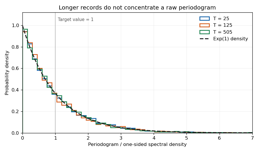
The figure uses the allowed cancellation , so the observations reduce to white noise. Orthogonal Fourier projections give the exponential law exactly at each plotted record length; increasing the record does not narrow the individual periodogram ordinate.
Past exam of the mathematics course of the University of Cambridge 2001 iii Paper 32 4 Solution by Codex 0 Created 2026-10-03 Updated 2026-10-14
Codex 0 Created 2026-10-03 Updated 2026-10-14An M-estimator based on an estimating equation chooses a consistent root ofIts population target solves . For a scalar parameter, suppose the root is locally unique andFor the contaminated distribution , differentiate its population equation at zero contamination. The influence function satisfiesConsequentlyThe constant of proportionality is independent of . A local expansion of the sample estimating equation similarly givesThe central limit theorem yields asymptotic normality with the sandwich variance of an M-estimatorThus the first-order variance of the unscaled estimator is . For a vector parameter the same differentiation gives and , with and .
For the location problem, take the target location to be zero and let have the standard normal distribution, with density and distribution function . An odd score has . For a differentiable score, integration by parts givesThe last expression also gives the appropriate derivative of the population equation for bounded monotone scores with jumps, by differentiating the shifted normal density. Assume and put . ThenMultiplying a score by a positive constant changes neither its estimator nor this normalized influence function.
First establish feasibility. The bound impliesso necessarily . For , let solveThis solution is unique: the ratio tends to as , tends to infinity as , and has positive derivative becauseTake the Huber score . Its derivative is one on and zero outside, so . HenceIt is odd, nondecreasing, meets the bound, and satisfies .
To prove optimality, put . For each fixed , the minimum of over is attained by projecting onto , which is exactly . Therefore every competing normalized influence function satisfiesTaking expectations, the right-hand side vanishes because both functions satisfy . Thus . This proves the optimal bounded influence function for normal location, even over the larger class of all bounded normalized functions, and hence over the required odd nondecreasing class. Its minimum asymptotic variance isThe numerator is .
At the included boundary , equality in the feasibility bound forces almost everywhere. This is the influence function of the sample median, with . It is obtained from the rescaled scores as . The boundary solution is the sign score, or equivalently the median estimator. Literal substitution of in the clipped score gives the identically zero function and no identifiable estimating equation; the printed clipped formula therefore requires this limiting interpretation at equality.
Pinned article: Introduction to the OurBigBook Project
Welcome to the OurBigBook Project! Our goal is to create the perfect publishing platform for STEM subjects, and get university-level students to write the best free STEM tutorials ever.
Everyone is welcome to create an account and play with the site: ourbigbook.com/go/register. We belive that students themselves can write amazing tutorials, but teachers are welcome too. You can write about anything you want, it doesn't have to be STEM or even educational. Silly test content is very welcome and you won't be penalized in any way. Just keep it legal!
Intro to OurBigBook
. Source. We have two killer features:
- topics: topics group articles by different users with the same title, e.g. here is the topic for the "Fundamental Theorem of Calculus" ourbigbook.com/go/topic/fundamental-theorem-of-calculusArticles of different users are sorted by upvote within each article page. This feature is a bit like:
- a Wikipedia where each user can have their own version of each article
- a Q&A website like Stack Overflow, where multiple people can give their views on a given topic, and the best ones are sorted by upvote. Except you don't need to wait for someone to ask first, and any topic goes, no matter how narrow or broad
This feature makes it possible for readers to find better explanations of any topic created by other writers. And it allows writers to create an explanation in a place that readers might actually find it.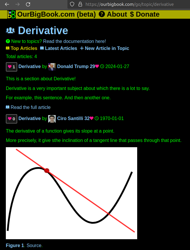
Figure 1. Screenshot of the "Derivative" topic page. View it live at: ourbigbook.com/go/topic/derivativeVideo 2. OurBigBook Web topics demo. Source. - local editing: you can store all your personal knowledge base content locally in a plaintext markup format that can be edited locally and published either:This way you can be sure that even if OurBigBook.com were to go down one day (which we have no plans to do as it is quite cheap to host!), your content will still be perfectly readable as a static site.
- to OurBigBook.com to get awesome multi-user features like topics and likes
- as HTML files to a static website, which you can host yourself for free on many external providers like GitHub Pages, and remain in full control

Figure 2. You can publish local OurBigBook lightweight markup files to either OurBigBook.com or as a static website.
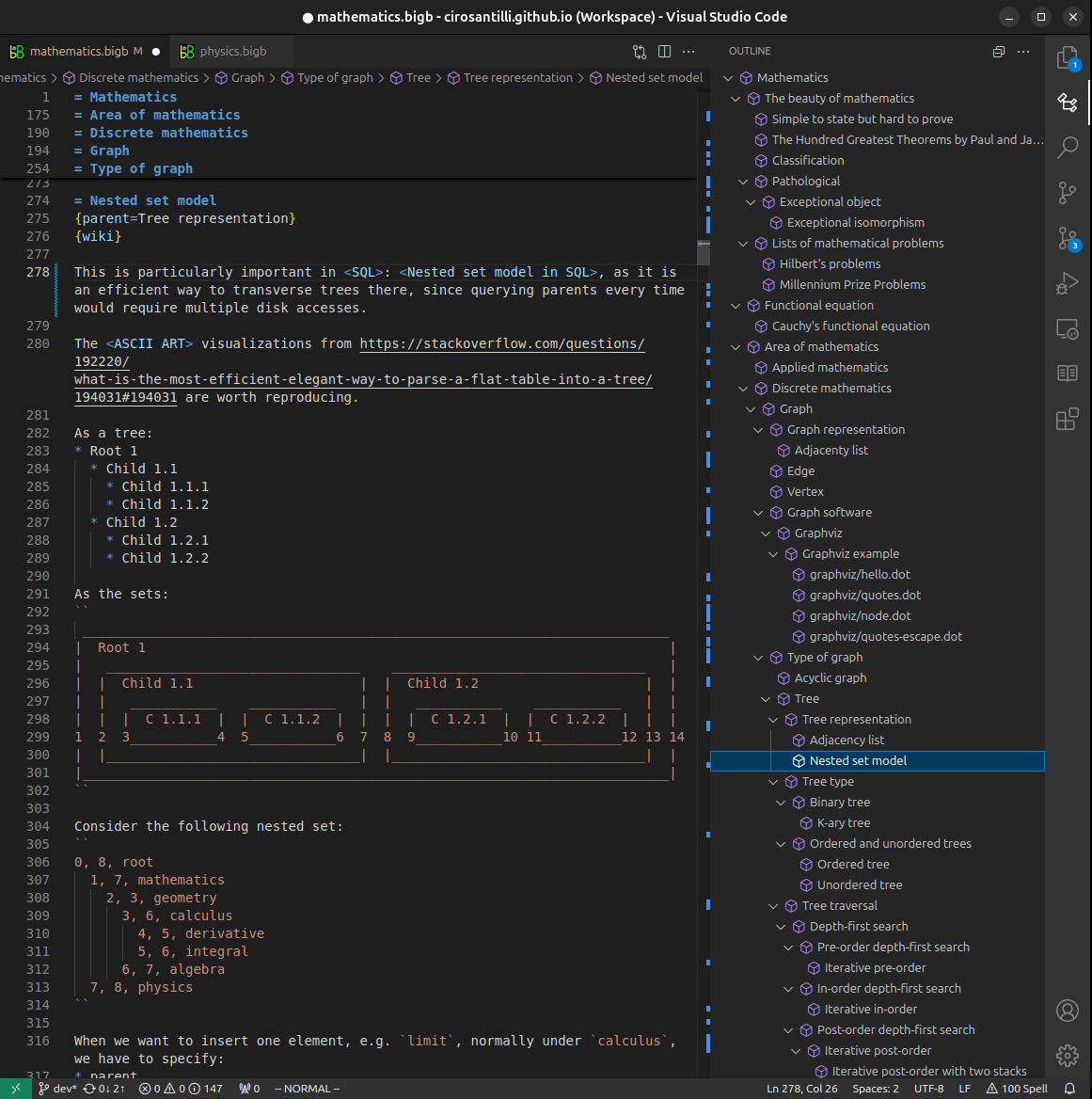
Figure 3. Visual Studio Code extension installation.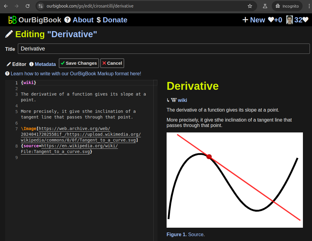
Figure 5. . You can also edit articles on the Web editor without installing anything locally. Video 3. Edit locally and publish demo. Source. This shows editing OurBigBook Markup and publishing it using the Visual Studio Code extension. 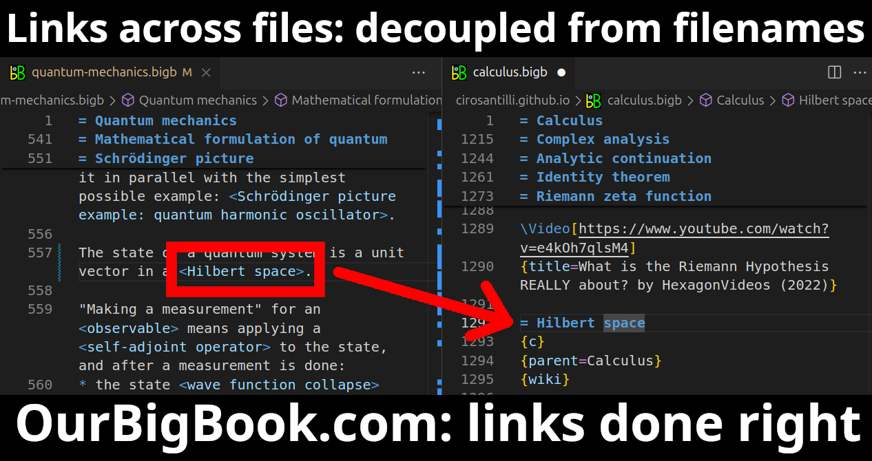
- Infinitely deep tables of contents:


All our software is open source and hosted at: github.com/ourbigbook/ourbigbook
Further documentation can be found at: docs.ourbigbook.com
Feel free to reach our to us for any help or suggestions: docs.ourbigbook.com/#contact