Topics (384k) Articles (398k) Users (410) Discussions (242) Comments (383) Files (13k) New article
For an exactly soluble example, set , , and . Start with zero electric currents, and apply a constant electric potential difference at . The sums and obey separate first-order linear differential equations:Their time constants are and . Thus, for ,Since , for , but as . The primary approaches . The secondary response opposes the rise of linked magnetic flux, in accordance with Lenz's law. Removing mutual inductance by setting makes the two exponentials equal and gives zero secondary electric current.
For stipulated , , and , the two time constants are and . Setting gives its largest negative magnitude atThe continuing primary electric current eventually reaches while the secondary returns to zero. These numbers belong to the stated model, not the 1831 apparatus.
Victor Franz Hess's 1912 series used two sealed, 3-mm-walled ionization chambers with Theodor Wulf's fiber electrometers. Karl Bergwitz suggested internal plating; Günther & Tegetmeyer improved focusing. Basket-mounted ground comparisons, insulation-loss measurements, simultaneous detectors and barograph-derived heights supplied checks. The highest flight reached 5350 m; its comparisons came from Vienna and after landing, without a launch-site baseline.[ref]
Über Beobachtungen der durchdringenden Strahlung bei sieben Freiballonfahrten by Victor Franz Hess. 1912, pp.1084-1085 apparatus and preparations; pp.1087-1088 seventh flight; English primary-text translation arxiv.org/pdf/1808.02927 pp.1-2, 5-6
A third, thin-walled chamber admitted ambient air. Hess multiplied its readings by , with pressure in millimeters of mercury, warning that vessel-wall contributions might violate this scaling. He recorded outside temperature but applied no absolute-temperature correction. Night flights, an eclipse and weather observations constrained alternatives to radiation from above; the eclipse argument addressed directly propagating solar radiation.[ref]
Über Beobachtungen der durchdringenden Strahlung bei sieben Freiballonfahrten by Victor Franz Hess. 1912, p.1085 pressure reduction; p.1086 eclipse; p.1088 temperature footnote; pp.1090-1091 inference; English translation pp.2-3, 6-8
The electrometers read gradual electric potential loss caused by continuing air ionization. The low-altitude dip and strong high-altitude rise favored an extraterrestrial contribution, without measuring proton composition.[ref]
Über Beobachtungen der durchdringenden Strahlung bei sieben Freiballonfahrten by Victor Franz Hess. 1912, pp.1089-1091 altitude averages and interpretation; English translation pp.7-8
An ionization chamber integrates electric charge: one energetic particle may create many ion pairs, several particles may contribute to one reading, and a photon can create charged particles in the gas or walls. A voltage-loss reading is therefore neither a count of primary cosmic rays nor a chemical analysis of them.Domenico Pacini supplied independent evidence: in June 1911 he compared a copper-box-enclosed electroscope at the sea surface and 3 m underwater, more than 300 m offshore above an 8-m-deep seabed. Reduced underwater ionization, stable electrical loss between runs, and a lake comparison supported an external contribution independent of soil radioactive decay. Water provided shielding; this established a different constraint from Hess's altitude comparison.[ref]
La radiazione penetrante alla superficie ed in seno alle acque by Domenico Pacini. Pacini's 1912 report, English translation pp.3-5, especially surface/underwater comparison and residual-ionization discussion; original Italian facsimile pp.9-14
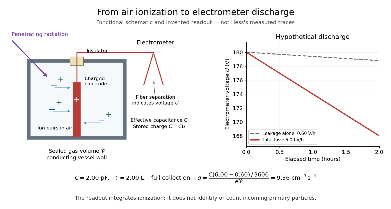
From air ionization to electrometer discharge
. Original functional schematic and invented readout example for the ionization-chamber charge-loss model. The chamber drawing is not a dimensional reconstruction, and the plotted voltage traces are not Hess's measurements. Details.An air shower is a cascade of secondary particles produced by an energetic particle interacting in the atmosphere. Both a charged particle and a gamma ray can start one.[ref]
Cosmic Rays: Particles from Outer Space by CERN. A new world of particles, secondary showers; Cosmic accelerators, gamma-ray showers
A secondary cosmic ray here is a particle produced by an atmospheric interaction of a primary cosmic ray or its descendants. A muon at ground level need not have traveled from the original astronomical source.
Convolution of a Cauchy distribution and a uniform distribution by  Codex 0 Created 2026-10-18 Updated 2026-10-20
Let have the Standard Cauchy distribution and let , independently, have the uniform distribution on , where . The convolution of probability densities gives the probability density of asThis is an even function. Its derivative isso its unique mode is zero. Its tails satisfy as : multiplying the integral by makes the integrand converge uniformly to on the bounded interval . Consequently both positive and negative parts of the first moment diverge, so its expected value does not exist. The symmetric Cauchy principal value of that moment is zero, which is a different assertion. Adding a bounded independent displacement smooths the probability density without removing the divergent first moment of the Cauchy distribution.
Use for the normal-state single-spin density of states per unit energy and volume at the Fermi surface. Write the attraction as , with , and define .[ref]
Theory of Superconductivity by John Bardeen and others. p.1182, equations (2.34)–(2.40), one-spin density of states; volume normalization stated here
Since has units of energy, has units of energy times volume, making dimensionless. Set , an energy cutoff using the Debye frequency , rather than a frequency itself. These conventions also fix the meaning of the earlier constant-shell BCS gap equation.
Here is the reduction of the BCS gap equation in these conventions. Substituting the zero-temperature BCS anomalous average givesThe sum counts one spin species. For , cancelling and replacing this sum by an integral with constant givesThe factor two from the symmetric integral cancels the in the BCS anomalous average; it is not an extra spin degeneracy. Substituting evaluates the integral as . Solving givesThe first equality is exact within the constant-density of states, sharp-cutoff mean-field approximation; the last is the weak coupling asymptote. Extending the first equality to large does not make this simplified model an accurate description of a strongly coupled material.
For an original numerical example, choose and . The exact constant-shell BCS gap equation gives ; the weak coupling formula gives . Its fractional underestimate, measured against the exact result, is exactly . At that error is , so the two formulas are no longer interchangeable. No material parameters have been fitted here.
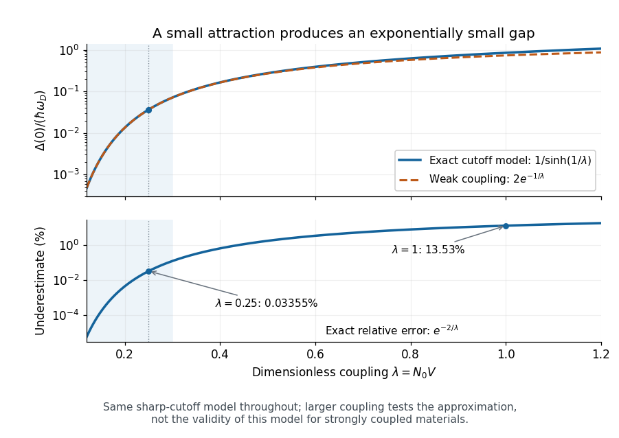
The exact cutoff gap and the range of the weak-coupling approximation
. Original zero-temperature constant-shell BCS gap equation calculation. The upper panel compares with ; the lower panel gives the exact fractional underestimate . The shaded interval is a chosen small-coupling illustration, not an experimental boundary. The large-coupling part tests the asymptote within the same model. Details.At nonzero temperature, substitute the finite-temperature BCS anomalous average instead. The same cancellation yieldsAt the superconducting transition temperature take the continuous limit. The integrand at then has the finite limiting value , so no divergent endpoint needs to be inserted into a numerical quadrature. For , the resulting integral gives and . These ratios concern the isotropic weak coupling model.[ref]
Microscopic Quantum Interference Effects in the Theory of Superconductivity by Leon Neil Cooper. 1972 lecture, thermodynamic properties of the ideal superconductor, pp.80–82
A nonzero pivot element can still be a poor numerical choice. Partial pivoting bounds the absolute values of the elimination multipliers by one in exact arithmetic, because each numerator is no larger than the selected denominator. This usually improves numerical stability, but does not prevent every possible growth of intermediate entries or guarantee accurate answers for every linear system.[ref]
2.6 Row pivoting. Fundamentals of Numerical Computation by Tobin A. Driscoll and others; §2.6.4, Example 2.6.6, equation (2.6.3) and concluding discussion: small-pivot instability and the limits of pivoting
To see the mechanism without depending on hardware, define a toy floating-point arithmetic model. The operator rounds an exact real number to the nearest value with three significant decimal digits; halfway cases choose the even final digit, and . Allow an unbounded exponent range. Round the inputs and the result of every addition, subtraction, multiplication and division separately; a product followed by a subtraction rounds twice. This is a prescribed arithmetic model, not a measurement of a physical computer. All inputs in the following original example are represented exactly:Without a row interchange, the elimination multiplier is . The last coefficient and right-hand side becomeTwo distinct exact values now have the same rounded representation. Back substitution therefore returnsThe small difference carrying information about was lost during elimination; the final subtraction only exposes that loss. Dividing by the tiny pivot element amplifies sensitivity to the lost information.
With partial pivoting, interchange the two rows, including their right-hand sides, to start from . Now , and the rounded updates areBack substitution gives and . Both paths round intermediate values, but only the first creates million-sized entries and then divides a lost difference by .
The true solution follows from the original second equation :Evaluate the linear-system residual against the original data in exact arithmetic, separately from the three-digit solve. With , the maximum norm, the results areThe respective relative linear-system residuals are and . Computing the diagnostic in higher precision matters: a check made only against the rounded reduced equations would miss the original error.
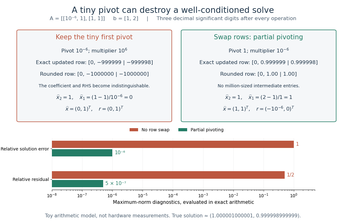
The same three-digit floating-point arithmetic model gives without a row interchange and with partial pivoting; exact linear-system residuals expose the difference
. Details. This matrix is well conditioned in the maximum norm: its induced matrix norm is , whileThe failure therefore belongs to this unpivoted algorithm, rather than a large condition number. In general, however, partial pivoting cannot remove sensitivity inherent in the data. For any approximate solution of an invertible matrix system, ; the induced matrix norm inequality and giveA small linear-system residual controls solution error only in conjunction with the condition number; numerical stability and sensitivity are different questions.[ref]
Substituting into the viscous Burgers equation gives . Integration permits the arbitrary function in the title. Multiplication of by preserves and reduces its equation to the heat equation. Thus the heat-equation representation uses a permissible time normalization rather than a condition uniquely imposed on every representative .
For a Planck function expressed as spectral radiance per frequency interval, is the Planck constant, the speed of light and the Boltzmann constant. Differentiating at fixed frequency givesThe proof uses and the chain rule. At low frequency, the multiplier tends to one, recovering the Rayleigh-Jeans law. At high frequency it grows approximately as : the same fractional temperature change has a larger fractional brightness effect on the declining spectral tail.
For an original example choose and . At , , so the first-order fractional residual is . At , , it is . Both spectra are exact blackbodies: this residual is a temperature mismatch, not evidence of a nonthermal spectrum. Fitting temperature before assessing remaining spectral residuals therefore removes a physically distinct degree of freedom. The figure divides by a fixed peak brightness rather than by the rapidly vanishing high-frequency tail.
An ideal differential measurement constrains two sky temperatures through . Represent every observed pair by a row of a matrix , with in column , in column and zeros elsewhere. Then and : adding any constant to the entire map changes no measurement. This null space is the angular angular monopole ambiguity, explaining why a directional comparison alone cannot measure the absolute blackbody temperature established by FIRAS.
For an original three-pixel example choose relative to an unspecified mean. Measurements and determine the third difference . The zero-mean condition recovers the chosen map, but adding to every pixel gives identical differences. The closure sum checks consistency without establishing the mean.
More generally, the graph joining measured pixel pairs must be a connected graph. If , each edge forces equal endpoint temperatures; a path propagates that equality throughout each connected component. Thus a connected observation graph leaves exactly one undetermined constant, whereas disconnected coverage leaves one per component. Fixing the mean makes an ideal connected reconstruction unique; real noise calls for least-squares solution fitting and uncertainty analysis.
The figure chooses a cosmic microwave background quadrupole sky , with and Legendre polynomial . On a great-circle scan, with measured from the chosen symmetry axis and ideal beams separated by ,Expanding proves the formula; its peak magnitude is . A constant sky gives zero. This deliberately restricted scan also misses some angular patterns, so rejecting the angular monopole is not a proof of complete sky reconstruction. Broad, overlapping coverage supplies the missing constraints; finite antenna beam patterns additionally smooth small angular features.
A hotter stellar core can favor a higher-barrier route despite fewer catalyst nuclei. To isolate this competition, prescribe a local hydrogen burning toy model at fixed mass density , with reference andChoose and , rounded barrier parameters for a proton pair and proton capture on nitrogen-14. These prescribe the temperature dependence, while the following freely chosen heating normalization incorporates effective nuclear factors and deposited energy:Here is hydrogen mass fraction, is CNO mass fraction, and is an arbitrary positive unit of stellar energy-generation rate. For and , the reference ratio is by construction. It is not a measured solar ratio. The CNO cycle bottleneck is represented by one effective rate, without evolving the existing proton-proton chain branches or catalyst network.
At , the logarithmic temperature slopes are and . The larger Coulomb barrier gives a steeper fractional response. Because these slopes change with temperature, this example retains the exponential rather than extending two fixed power laws. Writing and givesprovided the bracket is positive. With the chosen composition, . Reducing to at unchanged shifts it to . For , this catalytic route supplies no heat in this model. These are local toy crossovers: a whole star's luminosity requires integrating its stellar energy-generation rate through its stellar composition profile and stellar structure. Nuclear features, plasma screening and changes of the dominant bottleneck limit the model's extrapolation.
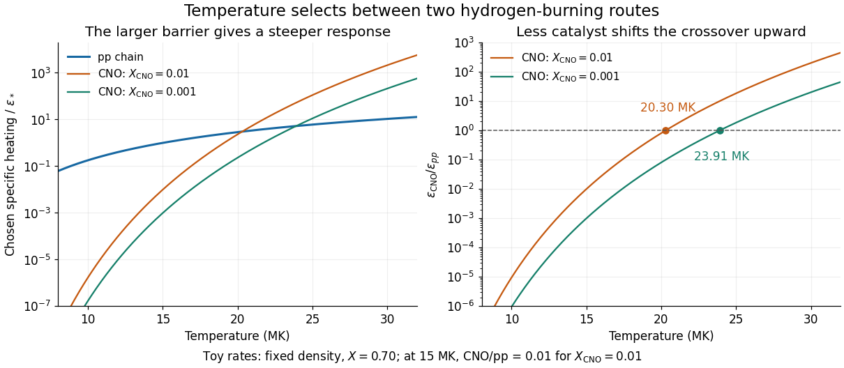
Chosen pp and CNO heating rates and their composition-dependent crossover
. Original local toy rates at fixed density and hydrogen mass fraction 0.70. The CNO-to-pp ratio at 15 MK is chosen as 0.01 for CNO mass fraction 0.01. Exponential barrier responses give crossovers at 20.30 and 23.91 MK for the two catalyst abundances. These are model curves, not stellar measurements or a fitted solar model. Details. Isentropic decompression of a spherical linear trap by Codex 0 Created 2026-10-18 Updated 2026-11-05
Codex 0 Created 2026-10-18 Updated 2026-11-05At fixed atom number, the entropy of the classical ideal gas in a spherical linear trap depends on temperature and strength through . Reversible adiabatic change therefore holds this product constant, giving the displayed relation. Reducing trap strength lowers the temperature while increasing cloud size. Its peak classical phase-space occupation remains constant, so this cooling alone does not make the gas more quantum degenerate. Heat exchange, particle loss or irreversible entropy production would change this relation.
Quantum degeneracy threshold in a spherical linear trap by Codex 0 Created 2026-10-18 Updated 2026-11-05
Codex 0 Created 2026-10-18 Updated 2026-11-05For a dilute classical trapped gas, with energy zero at the potential minimum. Thus . Quantum occupation effects begin when is no longer small, giving the displayed order-of-magnitude particle threshold. Equivalently, the central density satisfies . This is a degeneracy crossover criterion rather than an exact Bose condensation threshold. In the continuum approximation, spinless bosons have excited-state saturation , from the trap density of states proportional to . A quantum ground energy should be subtracted consistently when discreteness matters.
The clamped-beam Green function is symmetric. Its explicit formula depends only on and . More generally, two integrations by parts give when at both endpoints. Applying this identity to two point-load responses shows that the displacement at one point caused by a unit force at a second equals the displacement at the second caused by a unit force at the first.
For a positive-energy Dirac spinor normalized to unit probability and with positive helicity, the left-chiral component has squared weight , where in natural units. Its right-chiral weight is ; for negative helicity the two are exchanged. In an ultrarelativistic positive-helicity particle, the left-chiral amplitude is suppressed by a mass-to-energy ratio.
A charge carrier population per unit volume or, for a sheet, per unit area. The dimensional convention and whether different carrier species are counted separately must be specified.
X-ray fluorescence is Characteristic X-ray emission following excitation by incident photons. In a simple initially unexcited chemical atom, photoionization can eject an inner electron if the incident photon supplies its binding energy. An outer electron can then fill the vacancy, releasing an emitted photon with the difference of shell binding energies. Nonradiative relaxation competes with this route, so one absorbed incident photon need not yield one escaping characteristic photon.
Choose a separate stipulated electron shell model with values , and , all in . Ignore subshell splitting, recoil and changes of binding energy during relaxation. The possible shell differences areThese labels denote simplified shell groups, not resolved subshell electronic transitions. With , their calculated wavelengths are respectively , and . An incident photon exceeds both K-line energies but cannot directly create the K vacancy in this initially unexcited model. A photon can, leaving approximately of photoelectron kinetic energy. This comparison fixes neither the excitation probability nor the radiative branching probability.
X-ray emission spectroscopy studies the frequency spectrum of emitted X-rays. The spectral line positions identify electronic energy differences; their strengths also depend on excitation, photon absorption inside the sample, geometry and detector response. An X-ray tube may excite a sample with electrons, while X-ray fluorescence uses incident photons. The distinction matters when choosing what the experiment measures: identifying a chemical element from a line position is different from determining its abundance from a line strength.
For two ideal strings under a common tension, the positive mechanical impedances satisfy , where are their linear mass densities. The reflected fraction of incident power is . Solving for the positive ratio gives or its reciprocal. Squaring yields the displayed linear mass density ratios. For , the heavier string has times the lighter string's linear mass density; the impedance ratio is only .
Pinned article: Introduction to the OurBigBook Project
Welcome to the OurBigBook Project! Our goal is to create the perfect publishing platform for STEM subjects, and get university-level students to write the best free STEM tutorials ever.
Everyone is welcome to create an account and play with the site: ourbigbook.com/go/register. We belive that students themselves can write amazing tutorials, but teachers are welcome too. You can write about anything you want, it doesn't have to be STEM or even educational. Silly test content is very welcome and you won't be penalized in any way. Just keep it legal!
Intro to OurBigBook
. Source. We have two killer features:
- topics: topics group articles by different users with the same title, e.g. here is the topic for the "Fundamental Theorem of Calculus" ourbigbook.com/go/topic/fundamental-theorem-of-calculusArticles of different users are sorted by upvote within each article page. This feature is a bit like:
- a Wikipedia where each user can have their own version of each article
- a Q&A website like Stack Overflow, where multiple people can give their views on a given topic, and the best ones are sorted by upvote. Except you don't need to wait for someone to ask first, and any topic goes, no matter how narrow or broad
This feature makes it possible for readers to find better explanations of any topic created by other writers. And it allows writers to create an explanation in a place that readers might actually find it.
Figure 1. Screenshot of the "Derivative" topic page. View it live at: ourbigbook.com/go/topic/derivativeVideo 2. OurBigBook Web topics demo. Source. - local editing: you can store all your personal knowledge base content locally in a plaintext markup format that can be edited locally and published either:This way you can be sure that even if OurBigBook.com were to go down one day (which we have no plans to do as it is quite cheap to host!), your content will still be perfectly readable as a static site.
- to OurBigBook.com to get awesome multi-user features like topics and likes
- as HTML files to a static website, which you can host yourself for free on many external providers like GitHub Pages, and remain in full control

Figure 2. You can publish local OurBigBook lightweight markup files to either OurBigBook.com or as a static website.
Figure 3. Visual Studio Code extension installation.
Figure 5. . You can also edit articles on the Web editor without installing anything locally. Video 3. Edit locally and publish demo. Source. This shows editing OurBigBook Markup and publishing it using the Visual Studio Code extension. 
- Infinitely deep tables of contents:




All our software is open source and hosted at: github.com/ourbigbook/ourbigbook
Further documentation can be found at: docs.ourbigbook.com
Feel free to reach our to us for any help or suggestions: docs.ourbigbook.com/#contact