The dual space $V^{\ast }$ is the vector space of linear maps $V\to \mathbb{F}$, with pointwise operations. For the given basis define coordinate forms $e^i$ by $e^i({\sum }_j{a}_j{e}_j)=a_i$. These are linear and satisfy $e^i(e_j)={\delta }_{ij}$. If ${\sum }_i{c}_i{e}^i=0$, evaluation at $e_j$ gives $c_j=0$. For every linear form $\varphi$,so the coordinate forms span the dual and form its dual basis.

In the polynomial example write $p(X)=a+bX+c{X}^2$. ThenThese recover all three coefficients, so they span $V^{\ast }$ and, since the dual has dimension three, form a basis. Explicitly the basis dual to $1,X,X^2$ isEvaluation on the three monomials verifies the dual-basis identities directly.

Put $p(t)={\prod }_{j=1}^m(t-{\mu }_j)$ and define the Lagrange interpolation polynomialsTheir denominators are nonzero and ${\ell }_j({\mu }_i)={\delta }_{ij}$. The polynomial ${\sum }_j{\ell }_j-1$ has degree at most $m-1$ and vanishes at all $m$ distinct scalars, so it is zero. Suppose condition (a) holds, and put $E_j={\ell }_j(T)$. Since $(t-{\mu }_j){\ell }_j(t)$ is a constant multiple of $p(t)$,Thus each $E_{j}v$ lies in $V_j$, and every vector is a sum of such vectors. If ${\sum }_j{v}_j=0$ with $v_j\in V_j$, applying $E_i$ gives $v_i=0$, because ${\ell }_i(T)v_j={\ell }_i({\mu }_j)v_j$. Hence the sum is direct, proving (b). Conversely, on each $V_j$ the factor $T-{\mu }_{j}I$ vanishes; the factors commute, so $p(T)$ vanishes on every summand and therefore on $V$. This proves the equivalence without invoking primary decomposition.

If $ST=TS$ and $v\in V_j$, then $(T-{\mu }_{j}I)Sv=S(T-{\mu }_{j}I)v=0$, so $S[V_j]\subseteq V_j$. Conversely, if each summand is preserved, then on $V_j$ both $ST$ and $TS$ act as ${\mu }_{j}S$. They agree on all summands and hence on $V$. Therefore

For a nonzero principal part the discriminant $\Delta =b^2-ac$ classifies the equation: it is hyperbolic for $\Delta >0$, parabolic for $\Delta =0$, and elliptic for $\Delta <0$. These are the three definitions requested by the inline roman labels.

In the hyperbolic case the characteristic equation $a(dy{)}^2-2bdxdy+c(dx{)}^2=0$ gives two distinct real tangent directions. Locally, with suitably smooth coefficients, solve the corresponding characteristic ordinary differential equations to obtain two independent families of curves. Label their level sets $\varphi =\text{constant}$ and $\psi =\text{constant}$. Their gradients satisfyand the coordinate Jacobian is nonzero. The chain rule therefore eliminates $u_{\varphi \varphi }$ and $u_{\psi \psi }$. The remaining mixed coefficient $2[a{\varphi }_x{\psi }_x+b({\varphi }_x{\psi }_y+{\varphi }_y{\psi }_x)+c{\varphi }_y{\psi }_y]$ is nonzero: otherwise the invertible coordinate change would send the nondegenerate principal quadratic form to zero. Divide by this coefficient and absorb all first-order terms into $g$, giving $u_{\varphi \psi }=g(\varphi ,\psi ,u,u_{\varphi },u_{\psi })$. This canonical reduction is local; a global chart is not automatic.

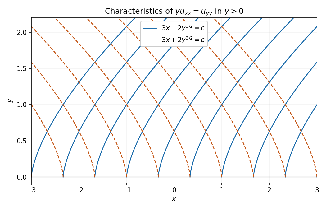
For the specific equation $a=y,b=0,c=-1$, so it is hyperbolic exactly on $y>0$, elliptic for $y<0$, and degenerate parabolic on $y=0$. For $\varphi =3x-2y^{3/2}$ and $\psi =3x+2y^{3/2}$, the Jacobian is $18\sqrt{y}\ne 0$. Direct differentiation givesSince $\psi -\varphi =4y^{3/2}$, the canonical form isThe characteristic families are $3x-2y^{3/2}=c$ and $3x+2y^{3/2}=c$, with slopes $dx/dy=\pm \sqrt{y}$. They are distinct for $y>0$ and meet the degeneracy line with coincident vertical tangent directions.

PutLeibniz differentiation gives $z^{\prime }=-{\int }_0^x\cos (x-s)f(s)ds$ and $z^{\prime \prime }=-f(x)+{\int }_0^x\sin (x-s)f(s)ds=-f-z$. Thus $z$ satisfies both zero initial conditions and the inhomogeneous equation. Every solution with $y(0)=0$ is $y=A\sin x+z(x)$.

On $[0,1]$, the second endpoint determines $A=-z(1)/\sin 1$ uniquely, since $\sin 1\ne 0$. Collecting the integrals, and using the sine addition formula for $s<x$, givesThis continuous kernel vanishes at the endpoints, satisfies $G_{xx}+G=0$ off $x=s$, and has derivative jump $-1$, as required for $-y^{\prime \prime }-y=f$. The preceding construction proves existence, and a homogeneous solution with both endpoints zero must vanish, proving uniqueness.

On $[0,\pi ]$, instead, the second boundary value becomesThus solvability is equivalent to ${\int }_0^{\pi }f(s)\sin sds=0$. When it holds, all solutions areThere is one free homogeneous mode because the endpoint length is resonant.

On $[-a,a]$ let $F=\Vert f{\Vert }_{\infty }$ and bound $|K|$ by $M$ on the compact integration region. Write $Th(x)={\int }_0^{x}K(x,s)h(s)ds$. The iteration gives $y_n={\sum }_{j=0}^n{T}^{j}f$. Induction, integrating absolute values also when $x<0$, givesThe exponential series is summable uniformly for $|x|\le a$. The Weierstrass M-test therefore proves uniform convergence to a continuous function $y$. Also $\Vert T(y_n-y){\Vert }_{\infty }\le Ma\Vert y_n-y{\Vert }_{\infty }\to 0$, so passing to the limit yields $y=f+Ty$.

For the indicated kernel, twice differentiating its integral givesConversely integrating the differential equation twice, with these initial conditions, gives the integral equation. This is valid also for negative $x$, either by oriented integration or by differentiating the double-integral identity.

For every finite $a$ the continuous kernel $(x-s)s$ meets the preceding hypotheses. Solutions on overlapping intervals agree: if $d=Td$ is their difference, iteration gives $\Vert d{\Vert }_{\infty }\le \Vert d{\Vert }_{\infty }(Ma{)}^j/j!$ for every $j$, forcing $d=0$. The solutions therefore patch to one solution defined on all of $\mathbb{R}$.

For $y^{\prime \prime }+p(x)y^{\prime }+q(x)y=0$, a singular point at zero is regular when $xp(x)$ and $x^{2}q(x)$ extend analytically to zero. Hereso these products are analytic at zero. The equation remains singular there because $q$ has a pole.

Substitute $y={\sum }_{n\ge 0}{a}_n{x}^{n+\sigma }$. The lowest power gives the indicial equation $\sigma (\sigma -1+\lambda )=0$. Comparing the next powers givesFor $0<\lambda <1$ the denominators do not vanish. With $\sigma =0$, $a_1=-a_0/\lambda$ and $a_2=0$, soWith $\sigma =1-\lambda$, the recurrence becomesConsequently $y_2=a_0{x}^{1-\lambda }(1-x{)}^{\lambda }$ on $0<x<1$, with the binomial series for its last factor. The nonzero coefficient ratios tend to one, giving radius one for that power-series factor. The factor $x^{1-\lambda }$ specifies the Frobenius branch; the different leading powers prove independence.

When $\lambda =1$, both indicial roots become zero and the analytic Frobenius solution in both cases is a multiple of $1-x$. To obtain the missing solution use reduction of order. Away from zero and one, $p=1/x$, henceThus the real general solution on any interval avoiding the singular points isIts Wronskian with $1-x$ is $1/x\ne 0$, proving independence. For complex solutions choose a logarithm branch on a suitable simply connected region.

Expanding gives $(I-E{)}^2-(I-E)=E^2-E$, so either operator is idempotent exactly when the other is. For an idempotent $E$,If $w\in \ker E\cap \mathrm{Im}E$, write $w=Eu$; then $0=Ew=E^{2}u=Eu=w$. Hence $V=\ker E\oplus \mathrm{Im}E$.

Next,If the right side vanishes, left multiplication by $E_1$ gives $E_1{E}_2+E_1{E}_2{E}_1=0$, while right multiplication gives $E_1{E}_2{E}_1+E_2{E}_1=0$. Subtraction shows $E_1{E}_2=E_2{E}_1$, and their original sum now gives $2E_1{E}_2=0$. Over the real or complex numbers this implies $E_1{E}_2=E_2{E}_1=0$.

For three idempotents summing to $I$, each pair sum equals the complementary idempotent $I-E_k$. Thus every product of distinct operators vanishes. Every vector equals $E_{1}v+E_{2}v+E_{3}v$. If $v_1+v_2+v_3=0$ with $v_i\in \mathrm{Im}{E}_i$, applying $E_j$ gives $v_j=0$. ThereforeTake a basis of each summand and unite the three bases. A vector in the $j$th basis has eigenvalue one for $E_j$ and zero for the other two, so this is the requested common eigenbasis. Zero summands simply contribute no basis vectors.

For a nonnegative integer $n$, put $z=e^{i\theta }$ on the unit circle. Since $\cos \theta =(z+z^{-1})/2$ and $d\theta =dz/(iz)$,The residue at zero is the coefficient of $z^{2n}$ in $(1+z^2{)}^{2n}$, namely $\left(\genfrac{}{}{0ex}{}{2n}{n}\right)$. The residue theorem givesThe contour integrand has no other poles. The formula also includes $n=0$, giving $2\pi$.