Topics (384k) Articles (398k) Users (410) Discussions (242) Comments (383) Files (13k) New article

Current-polarity dead-time compensation adjusts a switching command to oppose the dead-time output-voltage error predicted from the direction of load electric current. During bridge switching dead time, an inductive current can flow through a MOSFET body diode; the resulting rail clamp makes the cycle-average error depend on current direction. The manufacturer’s bridge-state diagrams establish that current-path mechanism.[ref]
Using power MOSFETs in DC motor control applications by Nexperia. IAN50004, §4.1, Figures 5–6: nonoverlap and body-diode recirculation
Consider an original ideal half-bridge model with rail separation , switching period , duty fraction , and effective dead-time fraction . Assume current has one nonzero sign throughout the affected interval and that device drops are negligible. Let positive current leave the midpoint, so that the adopted clamping model givesFor a desired normalized average , chooseSubstitution cancels the average error in this model. The correction changes the commanded pulse duration; it does not remove the nonoverlap needed to avoid H-bridge shoot-through. Different full-bridge switching patterns require applying the appropriate event model to each leg before subtracting the terminal averages.
For , and , and the uncompensated error magnitude is . At , use for positive current and for negative current. Each gives the intended average under the stated assumptions.
Command limits matter. Suppose the allowed duty range ends at because a minimum off-time is required. With positive current and , the formula asks for . Clipping to leaves an actual normalized average of , an error of at this bus potential difference. Thus a compensation law can be correct locally while the requested average lies outside its achievable range. Minimum pulse durations impose further limits.
Current-sign uncertainty in dead-time compensation is particularly important near a zero crossing. If an estimated sign is used while the actual sign is , the residual error, before command clipping, isA wrong opposite sign doubles the uncompensated error magnitude: in the example. Current-sensor delay, noise and a sign reversal within the switching interval can all invalidate a sign held constant for the cycle. Using a zero correction in an uncertain interval avoids that particular wrong-sign doubling, but does not cancel the original error.
A proposed bench comparison records gate commands, midpoint electric potential difference and load electric current together, then integrates each switching cycle with and without compensation. Compare positive-current, negative-current and crossing intervals separately, and repeat near pulse limits. This separates the average-error cancellation being tested from preservation of nonoverlap, device voltage drops and imperfect knowledge of switching delay.
Live-variable analysis computes which program variables may be read in the future before their current values are overwritten. It is a backward data-flow analysis: future uses make information flow toward earlier instructions. For a basic block , let contain values read before being defined in that block and let contain its definitions. ThenA value is needed on entry if the block itself first reads it, or if a successor needs it and the block does not replace it.[ref]
The LLVM Target-Independent Code Generator. Live Variable Analysis and Live Intervals
For a block
x = y + 1; return x;, y is live on entry but the old x is not. Iterating the equations over a finite control-flow graph yields a conservative answer useful for register allocation. Syntactically possible paths may include paths that execution can never take, so computed liveness need not prove that a use actually occurs.Illumination-initiation interaction in dye-loss controls tests whether changing illumination has the same response in the absence and presence of chemical initiation. A crossed factorial design separates the four conditions. For mean fractional losses , with indicating initiation and illumination, the contrastmeasures statistical interaction on the fractional-loss scale. In the STY-BODIPY assay context, the optical observable is carrier loss during co-autoxidation, not a direct label of its chemical cause.[ref]
A Continuous Visible Light Spectrophotometric Approach To Accurately Determine the Reactivity of Radical-Trapping Antioxidants by Evan A. Haidasz and others. Abstract: visible-light spectrophotometric co-autoxidation and kinetic/stoichiometric interpretation
The crucial qualification is response-scale dependence of dye-loss interactions. Consider an original first-order survival model with fully additive rate constants,ThenFor positive , and , this is negative even though the rates have no interaction term. With stipulated , in reciprocal time units and , the losses are , , and , giving . Saturation of fractional loss produces the contrast without a new chemical coupling.
On the transformed scale , the same noiseless model gives and zero interaction contrast. This transformation is appropriate only when the measured signal genuinely follows the stated survival model; product absorption or changing backgrounds can invalidate it. A transformed zero is therefore a conditional model check, not proof of a reaction mechanism.
For independent replicate measurements, the variance of the estimated loss contrast is . Four replicates per condition with common standard deviation 0.01 give a contrast standard uncertainty of 0.01. The modeled contrast above is smaller than that scale. Shared references instead introduce covariances that must be retained.[ref]
Match temperature, oxygen access, timing and readout exposure across conditions. Specify the response scale before interpreting a nonzero contrast as evidence about photobleaching or initiated oxidation.
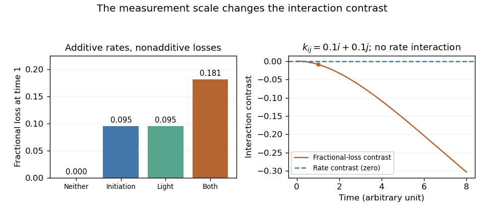
An original additive-rate model gives a negative interaction contrast on the fractional-loss scale. Transforming the same ideal observations back to rates gives zero rate interaction.
Details. Microbial culture preservation maintains recoverable cultures while retaining the biological properties needed for their future use. A successful preservation claim therefore concerns both viability and the identity or relevant characteristics of the recovered strain. It is part of the scientific function of a culture collection.[ref]
Guidelines for the Establishment and Operation of Collections of Cultures of Microorganisms by the World Federation for Culture Collections. section 7, preservation; section 8, checking recovered cultures
Approaches include microbial cryopreservation and freeze-drying. Their suitability depends on the material. ATCC's account explains that maintaining reference stocks can reduce the changes associated with repeated growth and passage, including changes caused by genetic instability and selection.[ref]
Mycology Culture Guide by ATCC. printed page 16, Preservation: reference stocks and phenotypic drift during prolonged passage
A toy selection model illustrates why repeated growth and preservation are different objectives. Begin with two variants A and B at equal abundance. Suppose each transfer multiplies their abundance ratio by in favour of A. After ten transfers the ratio is , making A's fractionBoth variants can remain viable while their proportions change from one half to about and . These invented values illustrate cumulative selection, not observed performance of a preservation method.
Recovery and comparison complete the scientific check. Obtaining growth shows that some material remains viable; confirming the intended genotype or phenotype asks another question. Records of origin, preservation history and characterization connect those observations. Separately maintained duplicates also protect a collection against loss of a single stored resource.[ref]
Guidelines for the Establishment and Operation of Collections of Cultures of Microorganisms by the World Federation for Culture Collections. sections 7.3 and 11, duplicate resources and documentation
Pinned article: Introduction to the OurBigBook Project
Welcome to the OurBigBook Project! Our goal is to create the perfect publishing platform for STEM subjects, and get university-level students to write the best free STEM tutorials ever.
Everyone is welcome to create an account and play with the site: ourbigbook.com/go/register. We belive that students themselves can write amazing tutorials, but teachers are welcome too. You can write about anything you want, it doesn't have to be STEM or even educational. Silly test content is very welcome and you won't be penalized in any way. Just keep it legal!
Intro to OurBigBook
. Source. We have two killer features:
- topics: topics group articles by different users with the same title, e.g. here is the topic for the "Fundamental Theorem of Calculus" ourbigbook.com/go/topic/fundamental-theorem-of-calculusArticles of different users are sorted by upvote within each article page. This feature is a bit like:
- a Wikipedia where each user can have their own version of each article
- a Q&A website like Stack Overflow, where multiple people can give their views on a given topic, and the best ones are sorted by upvote. Except you don't need to wait for someone to ask first, and any topic goes, no matter how narrow or broad
This feature makes it possible for readers to find better explanations of any topic created by other writers. And it allows writers to create an explanation in a place that readers might actually find it.
Figure 1. Screenshot of the "Derivative" topic page. View it live at: ourbigbook.com/go/topic/derivativeVideo 2. OurBigBook Web topics demo. Source. - local editing: you can store all your personal knowledge base content locally in a plaintext markup format that can be edited locally and published either:This way you can be sure that even if OurBigBook.com were to go down one day (which we have no plans to do as it is quite cheap to host!), your content will still be perfectly readable as a static site.
- to OurBigBook.com to get awesome multi-user features like topics and likes
- as HTML files to a static website, which you can host yourself for free on many external providers like GitHub Pages, and remain in full control

Figure 2. You can publish local OurBigBook lightweight markup files to either OurBigBook.com or as a static website.
Figure 3. Visual Studio Code extension installation.
Figure 5. . You can also edit articles on the Web editor without installing anything locally. Video 3. Edit locally and publish demo. Source. This shows editing OurBigBook Markup and publishing it using the Visual Studio Code extension. 
- Infinitely deep tables of contents:



All our software is open source and hosted at: github.com/ourbigbook/ourbigbook
Further documentation can be found at: docs.ourbigbook.com
Feel free to reach our to us for any help or suggestions: docs.ourbigbook.com/#contact