Topics (384k) Articles (398k) Users (410) Discussions (242) Comments (383) Files (13k) New article

A time-corrected electropherogram peak area is a raw electropherogram peak area divided by its migration time,It compensates for the longer passage time of a slower band through a concentration-sensitive detector in capillary electrophoresis. The first-party processing documentation defines this quantity explicitly and computes a percentage by dividing each corrected area by the sum of corrected areas.[ref]
The transport model explains the correction. If the baseline-subtracted detector signal is , internal capillary area is and band speed through the window is constant , thenWith detector distance and ,Thus dividing the time integral by migration time removes one speed dependence. It does not determine the response coefficient , injected sample amount or chemical identity.
For an original example, two peaks have raw areas 90 and 150 signal-seconds and migration times 150 and 300 s. Their corrected areas are 0.60 and 0.50 signal units. With equal detector response coefficients, their modeled relative amounts are , giving and of the corrected total. Raw-area normalization would instead give and .
Species-dependent detector response remains important. If the first coefficient is twice the second, amounts are proportional to and , giving and instead. Equal normalized corrected areas therefore need not mean equal amounts when the detector responds differently to the species. A measurement calibration must match the response and sample conditions being interpreted.
The reduction also assumes each band travels at a representative constant speed. If the electric field or electroosmotic flow changes substantially during a run, is an overall migration speed and need not equal the speed during detection. Baseline error, unresolved neighbors and nonlinear detector response are likewise not repaired merely by dividing by time. The software's chosen migration-time definition is part of the calculation: its CE mode uses the peak apex, while its CIA mode uses the midpoint of the start and end times.[ref]
A Schmitt trigger is a threshold circuit with hysteresis: its switching level depends on its current output state. An input rising through an upper threshold causes one transition, whereas an input falling through a lower threshold causes the reverse transition. Between the thresholds, the circuit retains the state reached previously. This makes a Schmitt trigger useful for turning a slowly varying or noisy signal into clean transitions, rather than repeatedly switching whenever noise crosses a single reference level.[ref]
Inverting Comparator With Hysteresis Circuit by Texas Instruments. SNOA997A, p. 1, Design Description; pp. 2–3, separate output-state equations
A simple inverting implementation puts the signal on the negative input of an electronic comparator. Connect its positive input to output through a resistor and to a reference through a resistor . Neglecting comparator input current, Kirchhoff's current law givesFor ideal high and low output levels , the input switches on a rise at and on a fall at . Thus the separation of the switching thresholds isThe output feeds back so as to reinforce its new state: after a rising input makes the output low, the positive-input threshold falls too.
For illustrative values , , , and , the thresholds are and . At an input of , the output can be either high or low, depending on the preceding trajectory. These chosen numbers describe the ideal circuit above, not a particular device specification.
An oscilloscope demonstration applies a slow triangular input with a small ripple and records input and output together. Compare the rising and falling transition levels, and then reduce the threshold separation to see when the ripple produces additional transitions. In a real circuit, input offset voltage, resistor tolerances, output loading and any internal hysteresis change the thresholds. An open-drain output also requires a pull-up resistor; its load must be included in the feedback calculation.[ref]
Inverting Comparator With Hysteresis Circuit by Texas Instruments. p. 1, Design Notes; pp. 2–3, pull-up and feedback network analysis
Band nonparabolicity is the departure of an energy band's dispersion relation from a quadratic function of crystal momentum near an extremum. A parabolic isotropic approximation writes , measuring from the band edge. Band coupling can make the apparent effective mass depend on energy, especially when the separation from another band is small.[ref]
Band structure of indium antimonide by Evan O. Kane. Abstract and pages 249–261: coupled conduction and valence bands in small-gap InSb
A useful isotropic model iswhere has units of inverse energy. A simple two-level illustration explains the extra factor: the eigenvalue above zero of a matrix with diagonal entries and real off-diagonal entry satisfies . Dividing by gives and . Real materials require a more detailed multiband model, including the appropriate symmetries and spin-orbit coupling.
Differentiating the model gives the group velocity and a momentum-to-velocity mass:This mass is distinct from the mass obtained from the local second derivative of . For , a state with parabolic estimate instead has . The energy grows more slowly than the band-edge parabola predicts. Evan O. Kane's 1957 InSb calculation connected such nonparabolic band coupling with measured optical absorption and cyclotron resonance data.[ref]
Band structure of indium antimonide by Evan O. Kane. Publisher abstract: absorption calculated using the cyclotron-resonance mass and compared with impurity-dependent absorption
An integrating amplifier produces an output proportional to the time integral of its input over an intended operating range. A common circuit uses an operational amplifier, an input resistor and a feedback capacitor . With the non-inverting input held at zero, ideal negative feedback maintains a virtual ground at the inverting input. Negligible amplifier input current then givesThe initial output records the capacitor's initial charge. Texas Instruments' circuit note derives this inverting relation and explains why real integration is limited by the circuit time constant and amplifier bandwidth.[ref]
For an original example, choose and , so . A constant0.20volt input lasting2milliseconds changes the output by . Repeating ten such pulses without intervening input or integrator reset changes it by in the ideal model. The output retains information about accumulated pulse area, rather than only the present input value.
A small offset also accumulates. With the same components, a residual input-equivalent1millivolt gives a slope of . Starting from zero, an idealized negative output limit at5volts would be reached in5seconds. The finite supply range causes amplifier clipping; an ideal integral extending indefinitely is not physically available.
Putting a resistor in parallel with the feedback capacitor supplies a DC path. Under ideal amplifier assumptions its zero-state transfer function isAt frequencies where , this approaches ; at low frequency it instead approaches the finite gain . The resistor prevents unrestricted DC accumulation while changing the lowest usable integration frequency.[ref]
An integrating amplifier can therefore turn a short detector pulse into a measurable accumulated output, but its initial condition, reset, baseline, frequency range and output limits belong to the measurement model. A charge amplifier is a related current-input arrangement in which collected charge is converted through feedback capacitance.
Amplifier clipping occurs when an electronic amplifier cannot follow the output amplitude predicted by its small-signal voltage gain. Its finite amplifier output range truncates the waveform. For a deliberately simple, instantaneous model with positive gain and fixed lower and upper output limits,Here and are input and output electric potential differences. The flat portions express a nonlinearity: doubling an already excessive input need not change the output. Real output limits depend on the supply, load and output stage. They need not equal the supply rails. Texas Instruments' example integrating amplifier uses separate supply and output-range design goals and explains how unrestricted DC integration eventually reaches saturation.[ref]
Integrator Circuit by Pete Semig. p1, Design Goals and Design Description
Amplifier clipping can corrupt an area measurement even when the waveform still looks easy to integrate. Suppose , , , and a rectangular input is for and zero otherwise. Its true area is , but the ideal unclipped output of is reduced to . Dividing the clipped waveform area by the gain gives50% below the true input area. Any rectangular input at or above with the same duration produces this same clipped plateau in the stipulated model. Subsequent integration cannot recover which of those input amplitudes was present.
A useful bench experiment feeds a repeatable pulse into an electronic amplifier and records both input and output on an oscilloscope. Increase the input amplitude while holding the gain, pulse duration and load fixed. The output first scales with the input, then ceases to do so near its limits. Reducing the gain tests whether an apparent input plateau is actually a receiver limit. Comparing measured areas before and after that change reveals the clipped waveform area bias directly.
The instantaneous clipping formula does not describe the internal dynamics of a saturated integrating amplifier. Once its feedback assumptions fail, recovery can take additional time. The ACF2101's historical datasheet explicitly distinguishes output overload from ordinary reset and describes extra recovery delay; the relevant behavior must be characterized for the actual circuit.[ref]
ACF2101 Low Noise, Dual Switched Integrator datasheet. p10, Output Overload
An integrator reset establishes a new starting state, while a suitable input range prevents information being lost before that reset.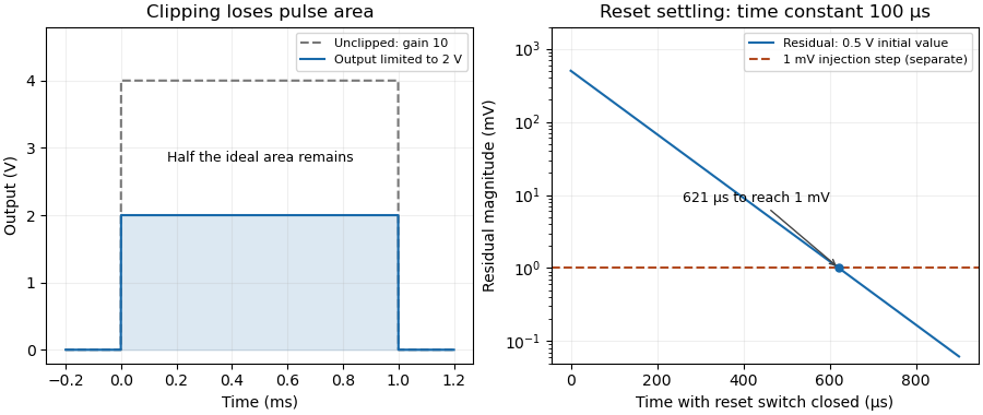
The amplifier output range is the interval over which an electronic amplifier can provide the specified output behavior under stated supply, load and operating conditions. Its limits need not coincide with the power-supply potentials. The historical integrator datasheet lists output range and output-current conditions separately from its supply conditions.[ref]
ACF2101 Low Noise, Dual Switched Integrator datasheet. Electrical Specifications, pp2–3, test conditions and Output section
For an original linear model, let with positive gain. Avoiding static clipping requiresStipulate a – supply, usable output limits –, and . The permitted differential input interval is to . A positive input predicts and fits; a negative input predicts and does not.
These are stipulated limits, not a product guarantee. The amplifier output headroom relative to each supply can differ. Loading can change the available output swing, and input-stage saturation can occur even when the final ideal output lies inside its range. A slow input sweep identifies the static departure from linear gain; a pulse test additionally probes dynamic recovery. Amplifier clipping describes the waveform consequence of exceeding these limits.
An instrumentation amplifier amplifies a differential input while presenting high input impedance and rejecting a common component. A useful ideal relation isIts common-mode rejection ratio describes finite unwanted response to common-mode voltage. This is distinct from the amplifier input common-mode range over which the circuit can operate without internal saturation.[ref]
A Practical Review of Common Mode and Instrumentation Amplifiers by Eamon Nash. Introduction; equations1–2 and Common Mode Voltage Range
For an original example, stipulate , , and . The differential signal is and the ideal output is , assuming all input and output limits are satisfied.
Now suppose the differential-to-common gain ratio is , or . The common-mode gain is then . A common-input change contributes at the output, five percent of the desired signal contribution. A high rejection ratio therefore does not mean zero error.
A source that changes both inputs together tests rejection; a source that changes their difference tests differential gain. Both tests must respect input common-mode limits, amplifier output range, load and frequency response. A plausible ideal output value alone does not prove that every internal stage remains linear.
Electronic gain expresses how an electronic circuit scales a specified input signal quantity into an output quantity. For a linearized voltage amplifier around its operating point, the voltage gain is . At a sinusoidal frequency it can be a complex phasor ratio, specifying both amplitude ratio and phase shift. Power gain instead compares the average power delivered to the load with the average signal power entering the amplifier:State the input/output quantities, frequency, load and operating conditions when specifying gain. A transimpedance amplifier relates output electric potential difference to input current and has a dimensional transfer ratio in ohms.
For an original circuit example, use an inverting operational amplifier with input resistor , feedback resistor and load . In its ideal negative-feedback linear regime,An input of root mean square therefore gives root mean square at the output, with a phase inversion. The manufacturer's primary explanation derives this resistance-ratio gain using the input and feedback currents.[ref]
Op-Amps, Comparator Circuit by Renesas. Op-Amp Basics (1), Figure 2 and the derivation of the inverting gain
Suitable supplies, output-current capability and amplifier output range are assumptions of this worked model, not specifications of a particular device.Here the input resistance is in the ideal model. For resistive ports and root-mean-square signal amplitudes,The example input power is and load power , giving . The additional output energy comes from the amplifier's supply, controlled by the input signal. The impedance condition for converting voltage gain to power gain is essential: voltage magnitude alone does not specify load power.
Voltage gain is conventionally expressed as decibels, while power gain uses . This example has voltage gain and power gain ; the two expressions agree when the resistive input and load impedances are equal. A negative voltage gain indicates phase inversion; its magnitude enters the logarithm.
A direct test drives a small sine wave into the input and measures the actual terminal signals with an oscilloscope. Sweeping frequency reveals the frequency response; increasing amplitude reveals amplifier clipping or other departure from the assumed linear gain. Keep the load and measurement impedances specified. Gain can amplify input noise along with signal, so the signal-to-noise ratio requires its own measurement.
The load impedance is the terminal electrical impedance of the receiving electrical load, at a stated frequency and operating condition. With electric current defined as entering the load's positive-voltage terminal, sinusoidal steady-state phasors obeyThe complex number records both the amplitude ratio and the phase difference. It belongs to the selected terminals and model; an arbitrary nonlinear device need not have a single amplitude-independent impedance.
A resistor gives . A series resistor and capacitor giveFor , and , this is about , with magnitude and phase . Load electric current leads its terminal electric potential difference in this example. The component laws and phasor interpretation follow the sinusoidal circuit model.[ref]
University Physics Volume 2 by Samuel J. Ling and others. Section 15.3, RLC series circuits and impedance
The load changes the source's operating point. A source with open-circuit phasor and series impedance suppliesFor RMS phasors, the complex power entering the load is . Its real part is the mean delivered power,Using peak rather than RMS amplitudes would introduce a factor in that power expression.
An original resistive example has RMS and . A load draws , receives and dissipates . A load instead receives and dissipates . More delivered power need not mean a smaller voltage error.
The input impedance of an instrument is a load when the instrument is connected to a source. High-input-impedance buffering reduces this interaction in voltage measurements.[ref]
Instrumentation amplifier (IA) topologies: three-amp by Tamara Alani. Presentation slides 3–5, source loading and input buffering
Impedance bridging prioritizes preserving the source signal; impedance matching addresses other objectives such as maximum power transfer under its assumptions.Impedance bridging, also called voltage bridging, connects a source to a much higher load impedance so that little signal electric potential difference is lost across the source's output impedance. It is useful when the receiver should observe a signal while drawing little electric current from its source.
Represent a linear source at one frequency by open-circuit phasor and series electrical impedance . With receiving input impedance , the voltage divider givesThus makes close to one as a complex number, controlling both amplitude and phase loading. For positive electrical resistances, the relative voltage loss is . A source feeding retains of its open-circuit voltage; feeding retains .
For a tolerance on that resistive relative loss,The often convenient ten-to-one ratio is therefore a chosen accuracy compromise, not a universal definition. A one-percent limit requires at least a ninety-nine-to-one ratio in this ideal resistive model. Voltage divider loading error gives the related loading problem when the source is itself a divider.
Impedance bridging with capacitive input explains why a large DC electrical resistance is not enough at every frequency. With source resistance and receiving in parallel with capacitance ,At and , the DC ratio is about . With , its magnitude at is only about . The capacitive path loads the source despite the high DC input resistance.
Texas Instruments' three-amplifier presentation motivates high-input-impedance buffering by explicitly showing that source current and nonzero source output impedance degrade accuracy.[ref]
Instrumentation amplifier (IA) topologies: three-amp by Tamara Alani. Presentation slides 3–5, PDF pp. 3–5
A buffer changes the load seen by the signal source; its own finite input and output behavior still matter.Impedance matching has a different objective in maximum-power-transfer applications. For a resistive source, choosing equal source and load resistances gives half the open-circuit voltage, whereas bridging seeks a ratio near one. Signal fidelity, delivered power and high-frequency transmission behavior require their appropriate models.
A free current is the part of the macroscopic electric current assigned to mobile or externally supplied electric charges, rather than to the bound motion represented by polarization and magnetization. In a conductor, drifting conduction electrons provide a familiar example.
In macroscopic Maxwell's equations, the free-current density appears as . Here is the magnetic field strength and the electric displacement field. The separation depends on the material model; the total microscopic charge motion remains the source of the electromagnetic field.
For a thin elastic plate interacting with a liquid interface, the elastocapillary length isHere is the plate's bending stiffness, the surface tension, Young's modulus, the thickness and Poisson's ratio. In this plate convention has units , while has units ; their ratio has units of length squared. The quantity is different from the gravity-dependent capillary length.
To see the balance, bend a portion of sheet of lateral size through an angle of order one. Its curvature is of order , so its bending energy scales as . The competing surface energy scale is . Their dimensionless quantity is the sheet elastocapillary energy ratioLarge means that the capillary energy scale is large relative to the bending energy scale. This dimensional analysis does not make a universal threshold for complete closure in capillary origami.[ref]
Capillary Origami: Spontaneous Wrapping of a Droplet with an Elastic Sheet by Charlotte Py and others. Equation1 and its dimensional argument
For chosen illustrative values and , the elastocapillary length is . A lateral size of gives , whereas gives . These are calculations with assumed parameters, not measurements of a particular material.
Two ways of changing size give opposite trends. Keep Young's modulus, Poisson's ratio and surface tension fixed, and let be a lateral scale factor. At fixed thickness, stays fixed and . If all sheet dimensions shrink in the same proportion, then , and . Halving lateral size alone decreases the sheet elastocapillary energy ratio fourfold; halving lateral size and thickness together doubles it. The phrase "smaller sheets" therefore needs a specified thickness rule.
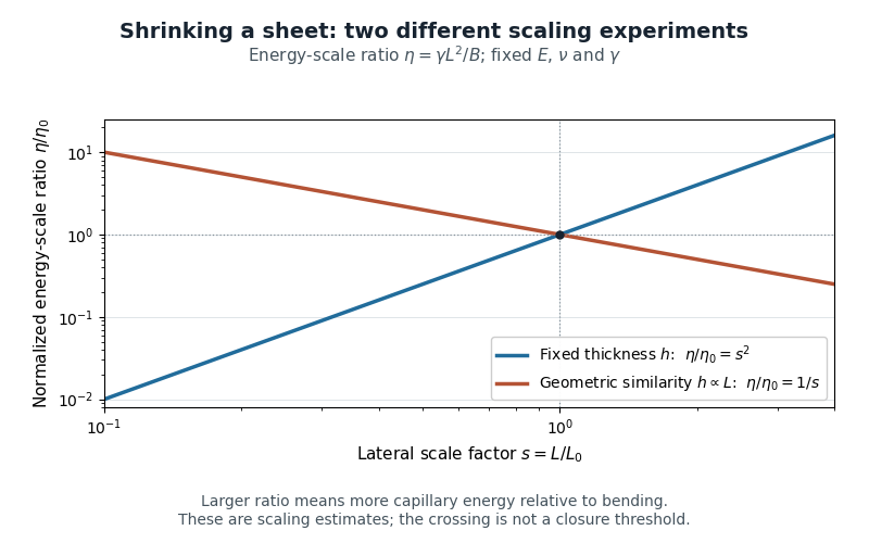
Changing lateral size at fixed thickness versus scaling all sheet dimensions: opposite trends in the capillary-to-bending energy-scale ratio
. Details. The length can also be calibrated directly: the 2007 study fitted an elastic-loop model to a long polydimethylsiloxane strip held by an ethanol meniscus. For their complete-wetting configuration, loop width was . The coefficient belongs to that model and geometry.[ref]
Capillary Origami: Spontaneous Wrapping of a Droplet with an Elastic Sheet by Charlotte Py and others. p.156103-2, Equation2 and loop-calibration paragraph
Capillary origami uses surface tension to fold an initially flat elastic plate around a liquid droplet. The fold trades a reduction in surface energy for an increase in bending energy; the initial outline helps select the resulting enclosure.[ref]
In the 2007 experiments of Charlotte Py and collaborators, 40–80 micrometre polydimethylsiloxane sheets rested on a water-repellent support. A water droplet reached the sheet's corners; time-lapse images followed its evaporation. Squares changed from four-corner bending to a tubular shape; triangles formed a tetrahedron. Smaller or thicker sheets could bend and then reopen without enclosing the droplet.[ref]
Capillary Origami: Spontaneous Wrapping of a Droplet with an Elastic Sheet by Charlotte Py and others. pp.156103-1–156103-2: preparation and square/triangular evaporation sequences
The elastocapillary length makes the thickness dependence quantitative. For fixed Young's modulus, Poisson's ratio and surface tension, the bending stiffness obeys and . Halving thickness therefore reduces by , about . At the same lateral size , the sheet elastocapillary energy ratio increases eightfold. This calculation explains why making the sheet thinner can enable wrapping even without changing its outline.
The sheet elastocapillary energy ratio compares available energy scales; it does not determine a unique final shape. The contact angle, initial liquid volume and outline also matter. A cut chosen to permit several panels to meet is a mechanical design choice, while the surface tension supplies the driving force. Predicting the complete folding path requires more than the scalar energy comparison. The same group reported cross-shaped templates forming a cube and flower-shaped templates forming nearly spherical enclosures.[ref]
The uniaxial sheet stretching stiffness is the coefficient relating axial force per unit width to axial engineering strain in a homogeneous thin elastic sheet under uniaxial stress with free lateral contraction. With Young's modulus and thickness ,Here for tensile force and sheet width . Since Hooke's law gives and , division by gives the result. has units , while has units .[ref]
Development of Constitutive Equations for Continuum, Beams and Plates by Tomasz Wierzbicki. §4.1, Equation4.1 and Figure4.1: uniaxial stress and lateral contraction
For an original example, choose , , and gauge length . Then . At strain , , and extension . The specimen's axial stiffness is , which depends on its width and gauge length.
A tensile measurement can infer from the slope of against . It needs known dimensions, reasonably uniform loading and freedom for lateral contraction; unloading tests elastic recovery. If lateral strain is instead constrained to zero while through-thickness stress remains zero, the plane stress equations give coefficient , with Poisson's ratio.[ref]
Development of Constitutive Equations for Continuum, Beams and Plates by Tomasz Wierzbicki. Equation4.16 and §4.2: plane-stress constitutive relations
The loading condition is part of the meaning of the reported stiffness.Elastic-rebound theory explains an earthquake as rapid release of elastic strain accumulated while a fault resists relative motion. When slipping occurs, nearby rock moves toward a less-strained configuration and part of the released energy propagates as seismic waves.
The motivating observations for the 1906 California earthquake included displacement across the fault and deformation away from it. H. F. Reid used those relationships to connect slow loading with sudden slip. The theory concerns stored deformation and its release; it does not imply that every fault is locked uniformly or that stress measurements alone predict an earthquake's time.[ref]
Reid's Elastic Rebound Theory by United States Geological Survey. 1906 observations and Reid's interpretation
Pinned article: Introduction to the OurBigBook Project
Welcome to the OurBigBook Project! Our goal is to create the perfect publishing platform for STEM subjects, and get university-level students to write the best free STEM tutorials ever.
Everyone is welcome to create an account and play with the site: ourbigbook.com/go/register. We belive that students themselves can write amazing tutorials, but teachers are welcome too. You can write about anything you want, it doesn't have to be STEM or even educational. Silly test content is very welcome and you won't be penalized in any way. Just keep it legal!
Intro to OurBigBook
. Source. We have two killer features:
- topics: topics group articles by different users with the same title, e.g. here is the topic for the "Fundamental Theorem of Calculus" ourbigbook.com/go/topic/fundamental-theorem-of-calculusArticles of different users are sorted by upvote within each article page. This feature is a bit like:
- a Wikipedia where each user can have their own version of each article
- a Q&A website like Stack Overflow, where multiple people can give their views on a given topic, and the best ones are sorted by upvote. Except you don't need to wait for someone to ask first, and any topic goes, no matter how narrow or broad
This feature makes it possible for readers to find better explanations of any topic created by other writers. And it allows writers to create an explanation in a place that readers might actually find it.
Figure 1. Screenshot of the "Derivative" topic page. View it live at: ourbigbook.com/go/topic/derivativeVideo 2. OurBigBook Web topics demo. Source. - local editing: you can store all your personal knowledge base content locally in a plaintext markup format that can be edited locally and published either:This way you can be sure that even if OurBigBook.com were to go down one day (which we have no plans to do as it is quite cheap to host!), your content will still be perfectly readable as a static site.
- to OurBigBook.com to get awesome multi-user features like topics and likes
- as HTML files to a static website, which you can host yourself for free on many external providers like GitHub Pages, and remain in full control

Figure 2. You can publish local OurBigBook lightweight markup files to either OurBigBook.com or as a static website.
Figure 3. Visual Studio Code extension installation.
Figure 5. . You can also edit articles on the Web editor without installing anything locally. Video 3. Edit locally and publish demo. Source. This shows editing OurBigBook Markup and publishing it using the Visual Studio Code extension. 
- Infinitely deep tables of contents:




All our software is open source and hosted at: github.com/ourbigbook/ourbigbook
Further documentation can be found at: docs.ourbigbook.com
Feel free to reach our to us for any help or suggestions: docs.ourbigbook.com/#contact