Topics (384k) Articles (398k) Users (410) Discussions (242) Comments (383) Files (13k) New article

A parabolic drag polar models drag coefficient as
The zero-lift drag coefficient supplies the intercept. In a simple finite-wing approximation, can represent lift-induced drag; fitted whole-aircraft values can include additional lift-dependent losses. The model is conditioned on a configuration and operating regime, rather than universally valid through aerodynamic stall.
The zero-lift drag coefficient supplies the intercept. In a simple finite-wing approximation, can represent lift-induced drag; fitted whole-aircraft values can include additional lift-dependent losses. The model is conditioned on a configuration and operating regime, rather than universally valid through aerodynamic stall.
Its dimensional form explains a useful speed tradeoff. In steady level flight let lift equal gravitational weight , with fixed mass density and wing area . Substitution of and yields
The first contribution grows with speed; the second decreases as the required lift coefficient falls. Differentiation gives the minimum-drag speed .
The first contribution grows with speed; the second decreases as the required lift coefficient falls. Differentiation gives the minimum-drag speed .
Minimizing required propulsive power instead gives
The minimum-power speed is therefore different from the minimum-drag speed in this model. For stipulated , , , and , the speeds are about and , respectively.
The minimum-power speed is therefore different from the minimum-drag speed in this model. For stipulated , , , and , the speeds are about and , respectively.
These are idealized level-flight comparisons of required propulsive power. Engine efficiency, allowable lift coefficients and a speed-dependent polar can move an operational optimum. Relating the result to minimum sink speed in unpowered flight requires the additional shallow-glide approximation; it does not identify minimum fuel flow for an arbitrary engine.
The zero-lift drag coefficient is the drag coefficient at for a stated configuration and flow condition. It is not necessarily the drag at zero angle of attack: a cambered airfoil can have a nonzero zero-lift angle of attack. In a simple parabolic drag polar, , the lift-dependent term vanishes there.[ref]
Induced Drag Coefficient by NASA Glenn Research Center. Total drag decomposition,
The zero-lift drag coefficient also need not be the smallest drag coefficient on a general polar. An original shifted parabolic drag polar,has minimum at , while . Confusing the intercept with the minimum loses the shift caused by the particular aerodynamic configuration.
A measurement should locate the state where the measured lift crosses zero, then evaluate or interpolate drag at that state using compatible references. Zero readings can be affected by balance tare and systematic error. Measurements at several nearby angles of attack distinguish a crossing from one apparently small reading.
For a complete aircraft, the coefficient can include skin-friction, pressure and component-interaction effects under the selected decomposition. A finite-wing term proportional to can vanish at zero lift without making those other sources of drag vanish. Holding constant while changing speed is itself an approximation if the Reynolds number, Mach number or flow state changes.
A shifted parabolic drag polar models drag coefficient with its minimum at a possibly nonzero lift coefficient:Here and in the header notation. The shift separates the coefficient at minimum drag coefficient from the zero-lift drag coefficient, which is .
For an original model, take , and . The coefficients at , and are 0.020, 0.018 and 0.026. The smallest drag coefficient occurs at , but that point does not maximize the lift-to-drag ratio.
Writing and differentiating givesFor positive lift coefficients the unrestricted optimum is thereforeThe last equality follows by multiplying by and using . In the example, and the maximum ratio is about 23.12. An allowed lift interval must still contain before that model optimum is physically attainable.
The model can also be fitted as the ordinary quadratic . When , completing the square gives , and . This makes the relation between a fitted quadratic and the shifted parameters explicit.
A wind tunnel can sample both sides of the proposed minimum while keeping flow conditions and normalization fixed. A small residual at sampled points does not establish accuracy through aerodynamic stall. Nor should automatically be identified as pure induced drag: the usual ideal finite-wing relation depends on , and a fitted shifted polar may combine several effects.[ref]
Viscous drag is resistance to relative motion arising from viscosity. It transfers momentum between a moving object and its surrounding fluid, with mechanical energy dissipated as heat.
For a rigid sphere of radius moving at speed through an unbounded Newtonian fluid with dynamic viscosity , Stokes law gives drag magnitude in the creeping-flow limit. The force opposes relative motion. This linear law requires a small Reynolds number; a quadratic drag law appropriate to other flow regimes cannot be substituted without checking the assumptions.
Lift-induced drag is the component of aerodynamic drag associated with the three-dimensional flow that supports a finite wing’s lift. The trailing vorticity produces downwash, changing the local relative-flow direction. A force approximately perpendicular to that local flow consequently has a component opposing the freestream motion. NASA’s primary account identifies the counter-rotating wingtip vortices and the downstream force component produced by their induced flow.[ref]
Induced Drag Coefficient by NASA Glenn Research Center. Air Pressure of a Wing and Induced Drag Coefficient
For a small induced angle , a force perpendicular to the local flow has freestream components and . Hence . This elementary projection explains why changing the flow direction can change drag even without adding direct viscous rubbing to that model.
A useful finite-wing model iswhere is wingspan, the wing reference area and the span efficiency factor. Use the same reference area in and , with . NASA gives this coefficient relation and aspect-ratio definition.[ref]
Induced Drag Coefficient by NASA Glenn Research Center. Drag Coefficient, displayed Cdi and AR equations
It is a model of the induced contribution, not a statement that total drag has only this dependence in every flow regime.An original fixed-lift calculation eliminates the coefficients:Take , , , , and . Then , , , and . The corresponding induced-power contribution is . Doubling the speed while holding lift, span, density and efficiency fixed reduces this modeled drag to about .
What is held fixed matters. At fixed instead of fixed lift, induced drag grows with dynamic pressure. The familiar inverse-square-speed conclusion above therefore cannot be transferred to a test that holds angle of attack or coefficient fixed while changing speed. Changes in efficiency, separation or compressibility can also invalidate the assumed comparison.
Lifting-line theory relates spanwise loading, trailing vorticity and induced velocities. The ideal planar minimum for fixed lift and span has elliptic span loading; this is a statement about the load distribution, not merely the outline of the wing. Total drag measurements also contain profile and other contributions, so fitting a total-drag curve does not automatically isolate .
A proposed wind-tunnel study measures force components and freestream conditions for several lift settings, while separately accounting for support loads, wall effects and profile drag. A downstream velocity survey tests the predicted downwash structure. Force balance alone observes total aerodynamic loads; the split into induced and other drag requires the additional flow information or a justified model. Report those assumptions before inferring an efficiency factor from the measured drag.
A sensitivity mass is a small calibrated mass added to a loaded weighing instrument to determine its response to a known mass increment. NIST's double-substitution procedure calls this a sensitivity weight and uses it to establish sensitivity under the conditions of the comparison.[ref]
Weighing by Double Substitution by National Institute of Standards and Technology. SOP4–2019, p3, Summary and apparatus; pp6–7, selection and use of sensitivity weight
It supplies a local input step rather than a new determination of the entire load from zero.Let an original comparator give indications before and after adding mass . For a stable linear response over that increment,where is another indication difference near that working load. A constant additive zero cancels from each difference; instrumental drift or load-dependent response need not cancel.
For original indications , and assigned sensitivity mass , the local response is about indication increments per milligram. A difference increments gives . Using only a nominal label instead would give . The assigned mass and its measurement uncertainty, rather than the nominal label alone, enter the comparison.
The added step must be large enough to resolve reliably but remain within the response region relevant to the unknown/reference comparison. NIST specifies selection criteria and regularly spaced observations; it also requires the standards to have valid calibration information.[ref]
Weighing by Double Substitution by National Institute of Standards and Technology. p1, prerequisites; p3, Summary; pp6–8, sensitivity selection and observations
Keep handling, settling and environmental conditions consistent. A sensitivity mass does not by itself cancel buoyancy, temperature effects or uncertainty in the main measurement standard. Those contributions remain in the full double substitution weighing model.Graded dose response describes how the magnitude of a defined biological effect changes with dose or concentration under a specified protocol. The observable can be an activity, force, concentration or other quantitative endpoint. It differs from quantal dose response, which records whether a specified criterion is met. The EPA’s primary terminology explicitly separates degree of response from incidence or probability.[ref]
IRIS Glossary by the United States Environmental Protection Agency. Dose-Response Assessment, Dose-Response Relationship and Endpoint entries
For an original saturating concentration-response model, writeThe plateau is an absolute response level, while is the maximum change above baseline. At , the response is halfway between baseline and plateau. If they are and response units, that midpoint is , not . Stating the baseline convention is essential when comparing midpoint parameters.
The graded mean also does not determine a binary responder fraction. Two original four-observation examples, and , both have mean . With a response criterion of at least , their responder fractions are and . Converting a continuous measurement into a binary outcome discards information about response magnitude.
A controlled assay measures matched concentrations at stated observation times with suitable baseline and reference conditions. Pharmacokinetics can make an administered dose produce different concentration histories, and biological time dependence can change the effect even at the same nominal concentration. ICH-E4 discusses concentration-response information and the interaction of response with time.[ref]
Dose-Response Information to Support Drug Registration by ICH. Sections I.C and I.E, concentration-response data and time
A fitted curve is a model for the observed endpoint, not proof of a particular receptor mechanism. An apparent plateau may instead reflect an instrument limit or the tested range. Graded dose response is most useful when the measured quantity, normalization, exposure definition and uncertainties are all explicit.
Quantal dose response describes the probability or proportion of subjects meeting a specified binary response criterion at each exposure level. The response is yes/no for that criterion, rather than the magnitude of the underlying change. A curve therefore requires both the exposure definition and the endpoint used to classify a responder.[ref]
IRIS Glossary by the United States Environmental Protection Agency. Dose-Response Assessment and Endpoint entries
Let be when subject meets the criterion at dose and otherwise. The population quantity isUnder independent subjects with the same probability, has a binomial distribution. With responders among subjects, the estimate is and its plug-in standard error isThat is a sampling calculation, not a claim that each person has a effect magnitude or that the estimate is exact.
An original threshold model illustrates a possible origin of the curve. Suppose subjects have response thresholds , with response occurring when . Then , a cumulative distribution function. Equal proportions with thresholds , , and arbitrary dose units give a responder fraction at dose . Those subjects’ effect magnitudes are still unspecified. Real response need not follow a deterministic threshold for each person.
A dose associated with responders is consequently not the same parameter as a dose producing half a maximum graded dose response. Changing the responder criterion changes the quantal curve even if the underlying observations do not change.
The study design must handle observation time, population composition and repeated measurements. Several observations from one person are not automatically independent extra subjects. ICH-E4’s distinction between individual and population-average dose-response information is relevant to interpreting the resulting curve.[ref]
Dose-Response Information to Support Drug Registration by ICH. Section I.B, individual and population-average relationships
The curve summarizes a defined population and endpoint rather than supplying an individual dosing rule.The velocity-time integral is the area under a velocity-versus-time curve over a specified interval:It has units of length. In Doppler echocardiography, a systolic flow-velocity trace can be integrated to estimate the distance associated with that measured waveform. The interval, sampling site and method of tracing the spectrum are part of the measurement.
The exact volume transported through an opening isFor constant area and a representative area-mean normal velocity , this reduces to . Approximating the left ventricular outflow tract as circular then giveswhere is the measured diameter, SV is stroke volume, HR is heart rate and CO is cardiac output. The primary Doppler study relates integrated velocity and anatomical area to cardiac output and compares the result with independent methods.[ref]
Determination of cardiac output by Doppler echocardiography by Halfdan Ihlen and others. Theory and Abstract: velocity integration, aortic size and method comparison
For stipulated and VTI , the estimated stroke volume is . At 75 beats per minute, cardiac output is approximately . A triangular waveform with peak and duration has that same integral. A trapezoidal waveform with the same peak and duration, but 0.10-second rise and fall, has integral instead.
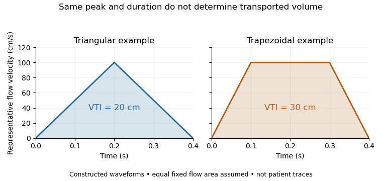
Equal peak flow velocities with different velocity-time integrals
. Details. The calculation depends quadratically on diameter: a 5% diameter overestimate produces a 10.25% area overestimate at fixed VTI. Flow-profile mismatch in Doppler stroke-volume estimation is a different error: a peak spectral envelope need not equal the area-mean velocity required by the volume integral. A VTI is also not automatically the path length travelled by one identifiable blood cell, since a fixed sampling region can observe different cells over time.
Pulsed-wave Doppler echocardiography uses timed ultrasound transmissions and returns to measure motion within a selected sampling region of the heart or nearby vessels. An echo's round-trip delay provides depth information, so a time window can select a location. The resulting Doppler spectrum describes a finite sample volume rather than an exact point.[ref]
Recommendations for Quantification of Doppler Echocardiography by Miguel A. Quiñones and others. General Principles, p.167; PW Doppler, pp.168–169
For sound speed and round-trip delay , the ideal depth is . Avoiding ambiguity between successive pulses in a simple single-depth system requires waiting at least before the next pulse. If is the pulse repetition frequency, this givesThe Doppler signal is sampled once per pulse, so unaliased shifts obey . For aligned flow and transmitted frequency ,This is the pulsed Doppler depth-velocity tradeoff in the stated idealization. With , and , the highest ideal pulse rate is and the corresponding speed limit is about . Doubling the depth halves both limits. Practical timing margins can reduce them further.
Aliasing is an ambiguity of the sampled signal, not proof that blood reverses direction. For example, sinusoidal Doppler shifts of and have identical complex samples at a pulse rate, because their frequencies differ by exactly one sampling rate. The example concerns the Doppler signal, not direct sampling of the megahertz acoustic carrier.
High-pulse-rate variants can trade unique range localization for a larger velocity range. Continuous-wave Doppler echocardiography instead transmits and receives continuously, accepting depth ambiguity. The choice of acquisition method therefore changes what information the measured spectrum contains.[ref]
Recommendations for Quantification of Doppler Echocardiography by Miguel A. Quiñones and others. General Principles and high-PRF discussion, pp.167–168
Continuous-wave Doppler echocardiography measures the Doppler frequency distribution of continuously transmitted and received ultrasound through the heart. It can record high flow velocities without the pulse-repetition-frequency aliasing limit of pulsed-wave Doppler echocardiography, but it does not select one depth along the beam. Signals from different contributing locations can overlap.[ref]
Recommendations for Quantification of Doppler Echocardiography by Miguel A. Quiñones and others. General Principles, printed p.167; CW Doppler, p.169
For an aligned flow at speed , the leading Doppler ultrasound relation isWith stipulated transmitted frequency , sound speed and , the shift is approximately . A pulsed measurement with pulse repetition frequency would have a Doppler Nyquist frequency of only . Continuous-wave acquisition avoids that particular pulse-rate restriction. Its receiving electronics and digital sampling still have finite bandwidth; continuous transmission does not imply unlimited measurable frequency.
The price is Doppler range ambiguity. If a beam intersects two moving regions, a peak in the spectrum does not by itself label which depth produced it. The anatomical image, direction, timing and waveform context supply additional evidence. The outer spectral envelope describes the fastest detected motion along the beam, rather than a direct spatial average over one known vessel opening.[ref]
Recommendations for Quantification of Doppler Echocardiography by Miguel A. Quiñones and others. CW Doppler, p.169, outer envelope and anatomical localization
This matters when estimating stroke volume. Multiplying a continuous-wave peak-velocity integral by an arbitrarily selected area can combine measurements from different sites or different parts of a velocity distribution. Flow-profile mismatch in Doppler stroke-volume estimation explains the separate requirement that the chosen velocity represent the area used in the volume calculation.
Color Doppler overlays spatially localized estimates of motion on an ultrasound image. In blood-flow imaging, the estimated quantity is related to the Doppler ultrasound shift of echoes from moving red blood cells. The color scale encodes motion relative to the beam, not the blood's oxygen content. The displayed legend and sign convention must be read with the image.[ref]
Recommendations for Quantification of Doppler Echocardiography by Miguel A. Quiñones and others. General Principles, printed p. 167, multiple gates and color velocity estimates
An important implementation estimates the phase change between repeated echoes using autocorrelation. Chihiro Kasai and coauthors demonstrated an autocorrelator combined with pulsed acquisition, testing scanners with phantoms as well as examining hearts. This made many localized estimates available fast enough for a changing two-dimensional image; it did not make each colored pixel an independent direct measurement of transported blood volume.[ref]
Real-Time Two-Dimensional Blood Flow Imaging Using an Autocorrelation Technique by Chihiro Kasai and others. Abstract and Sections II–III, mean Doppler frequency, system and phantom experiments
For an original single-frequency example, let successive complex echo samples be . Thenwhere is the Doppler ultrasound frequency shift and the pulse repetition frequency. The measured phase is unchanged when increases by any integer multiple of . This is aliasing even for a noiseless signal.
With Hz and transmitted frequency MHz, assume speed of sound m/s and motion parallel to the beam. True velocity 0.80 m/s gives Hz. Its principal sampled value is approximately Hz, corresponding to displayed beam velocity m/s under the same conversion. A color sign change can therefore occur without physical reversal of fluid flow.
The example isolates sampling. Mixed moving scatterers, finite spatial resolution and signal processing add further limitations. A color image is useful for locating a jet or a changing flow pattern, while a stroke volume requires an appropriate spatial and temporal integration of velocity, not the apparent size or brightness of a colored patch.
Bacteriophage T4 DNA polymerase is a DNA polymerase associated with bacteriophage T4. It extends an existing paired strand end in the direction using a DNA template and deoxynucleoside triphosphates. A primer supplies the extendable end. The enzyme also has exonuclease activity, supporting DNA polymerase proofreading; the characterized enzyme lacks a exonuclease function.[ref]
T4 DNA Polymerase by New England Biolabs. Product Information: synthesis direction, template/primer requirement and exonuclease activities
Extension and removal are competing chemical outcomes, not contradictory strand directions. A simplified kinetic example assigns rates and to two possible exits from one enzyme–strand-end state. If both exits have exponential waiting times, the probability that extension happens first isStipulated rates and give ; rates and give approximately . These illustrative numbers show how slowing extension relative to removal can favor proofreading. They are not measured constants for this enzyme or a complete model of its active-site transitions.
The same protein also supplied a historical binding target. In their 1990 primary study, C. Tuerk and L. Gold selected RNA sequences that bound T4 DNA polymerase, finding distinct selected sequences with equivalent binding constants.[ref]
Systematic evolution of ligands by exponential enrichment: RNA ligands to bacteriophage T4 DNA polymerase by C. Tuerk and L. Gold. Abstract: eight-base variant region and two selected RNA binders
Measuring binding to a protein and measuring its catalytic DNA synthesis answer different experimental questions. The selected RNA is an aptamer; it is not itself the polymerase. Pinned article: Introduction to the OurBigBook Project
Welcome to the OurBigBook Project! Our goal is to create the perfect publishing platform for STEM subjects, and get university-level students to write the best free STEM tutorials ever.
Everyone is welcome to create an account and play with the site: ourbigbook.com/go/register. We belive that students themselves can write amazing tutorials, but teachers are welcome too. You can write about anything you want, it doesn't have to be STEM or even educational. Silly test content is very welcome and you won't be penalized in any way. Just keep it legal!
Intro to OurBigBook
. Source. We have two killer features:
- topics: topics group articles by different users with the same title, e.g. here is the topic for the "Fundamental Theorem of Calculus" ourbigbook.com/go/topic/fundamental-theorem-of-calculusArticles of different users are sorted by upvote within each article page. This feature is a bit like:
- a Wikipedia where each user can have their own version of each article
- a Q&A website like Stack Overflow, where multiple people can give their views on a given topic, and the best ones are sorted by upvote. Except you don't need to wait for someone to ask first, and any topic goes, no matter how narrow or broad
This feature makes it possible for readers to find better explanations of any topic created by other writers. And it allows writers to create an explanation in a place that readers might actually find it.
Figure 1. Screenshot of the "Derivative" topic page. View it live at: ourbigbook.com/go/topic/derivativeVideo 2. OurBigBook Web topics demo. Source. - local editing: you can store all your personal knowledge base content locally in a plaintext markup format that can be edited locally and published either:This way you can be sure that even if OurBigBook.com were to go down one day (which we have no plans to do as it is quite cheap to host!), your content will still be perfectly readable as a static site.
- to OurBigBook.com to get awesome multi-user features like topics and likes
- as HTML files to a static website, which you can host yourself for free on many external providers like GitHub Pages, and remain in full control

Figure 2. You can publish local OurBigBook lightweight markup files to either OurBigBook.com or as a static website.
Figure 3. Visual Studio Code extension installation.
Figure 5. . You can also edit articles on the Web editor without installing anything locally. Video 3. Edit locally and publish demo. Source. This shows editing OurBigBook Markup and publishing it using the Visual Studio Code extension. 
- Infinitely deep tables of contents:



All our software is open source and hosted at: github.com/ourbigbook/ourbigbook
Further documentation can be found at: docs.ourbigbook.com
Feel free to reach our to us for any help or suggestions: docs.ourbigbook.com/#contact