Topics (384k) Articles (398k) Users (410) Discussions (242) Comments (383) Files (13k) New article

For an integer , the generalized divisor function counts ordered factorizations of a positive integer into positive integer factors. If , thenTo prove the formula, distribute the exponent among the factors. The number of nonnegative exponent tuples with that sum is the stars and bars count, and different primes can be assigned independently.
Thus and is the ordinary divisor function. For , . The ordered condition matters: exchanging two unequal factors changes the counted tuple. Absolute convergence for permits multiplying Dirichlet series, giving and connecting these counts with powers of the Riemann zeta function.
The closed graph ball of radius centered at vertex iswhere is shortest-path distance. In an unweighted graph, distances count edges, so a noninteger radius gives the same set as its integer part. Vertices in other connected components have infinite distance and lie outside every finite-radius ball.
For the path , and is the whole vertex set. The sphere at radius one contains only ; a ball also contains its center and all smaller distances.
Semidiscretization discretizes some variables of a differential equation while leaving others continuous. A spatial discretization of the heat equation gives interior grid values satisfyingBoundary values complete this ordinary differential equation system; time has not yet been replaced by a sequence of steps.
Applying explicit Euler later gives a fully discrete method with stability restriction for the standard uniform-grid diffusion model. Keeping the two stages separate makes spatial approximation error distinct from time-integration error and allows a different time solver to be used with the same spatial operator.[ref]
Finite Difference Computing with PDEs by Hans Petter Langtangen and Svein Linge. Chapter 3, spatial second differences and time-stepping diffusion
An incircular net in the Euclidean plane is formed by two indexed families of straight lines and such that each elementary quadrilateral bounded by has a common circle tangent to its four side lines. In the usual nondegenerate convex setting this is an incircle. The line families make the rows and columns straight; a mesh of unrelated tangential quadrilaterals is a more general object.[ref]
The square grid is an example, with one incircle centred in every square. A rectangular grid of unequal side lengths fails: a circle tangent to both horizontal sides must have radius half the height, while tangency to both vertical sides requires radius half the width. This simple test illustrates that the tangency constraint carries metric information. Checkerboard variants impose the condition on alternating cells and use oriented contact in Laguerre geometry.
Coherent sampling records an integer number of cycles of a periodic signal in the observation interval used for a discrete Fourier transform. For equally spaced samples at sampling rate , a single sinusoidal frequency is coherent whenThis is a frequency-and-record-length condition, not merely starting the acquisition at a particular phase.[ref]
Coherent Sampling vs. Window Sampling by Analog Devices. What Defines Coherent Sampling?, integer-cycle relation
For the complex tone , the unnormalized discrete Fourier transform givesA real cosine has the corresponding positive- and negative-frequency bins. The cancellation follows from a finite geometric sum; arbitrary phase does not spoil it. Periodic continuation means , not that the last stored sample must equal .
For example, and make a tone coherent, while is off the DFT grid. The latter's rectangular window record generally has spectral leakage into multiple bins. The bin spacing remains in both cases: coherence has not changed the grid spacing or increased the record duration.
Choosing relatively prime to can help an analog-to-digital converter test sample more distinct input phases, but it is an additional condition. A -cycle tone in samples is coherent even though its sampled phases repeat after only samples. The manufacturer's application note discusses the irreducible-ratio choice separately from the integer-cycle equation.[ref]
Coherent Sampling vs. Window Sampling by Analog Devices. Figure 1 explanation, cycle count and irreducible ratio
An experiment must also maintain the required ratio over the record. Frequency drift or clock variation can invalidate a nominal setting. If coherence cannot be maintained, a different window function can reduce leakage, with changes to amplitude scaling and spectral spread accounted for through the coherent gain of a window.
The unit rank of a number field is the rank of the free abelian part of the unit group of its ring of integers. If has real embeddings and conjugate pairs of complex embeddings, Dirichlet's unit theorem giveswhere is the finite group of roots of unity in . Hence the unit rank is .[ref]
The rational numbers and imaginary quadratic fields have rank zero; real quadratic fields have rank one. In , the unit has norm and its powers produce infinitely many units. The logarithms of the absolute embedding values of a unit sum to zero when complex pairs are counted twice. This places their logarithmic images in a hyperplane of dimension , explaining the geometric meaning of the rank.
A vertex is a descendant of in a directed graph when a directed path leads from to . Under the reflexive convention, a length-zero path makes its own descendant; a strict-descendant convention excludes that case and must be stated. An ancestor reverses this reachability relation.
For , the descendants of are under the reflexive convention, while is not a descendant of . In a directed cycle, distinct vertices can each be descendants of the other. Thus descendant reachability is transitive and reflexive but need not be antisymmetric.
In a directed acyclic graph, mutual reachability forces equality, so reachability defines a partial order. This makes descendant sets useful in dependency and causal graphs, while the graph alone still needs a specified interpretation before an arrow denotes causation.
An aliquot-aware dye inventory accounts for dye removed in samples as well as dilution by titrant. In dipyrrin titration mass balance, an absorbance change can result from changing protonation, changing solution volume or loss of material from the vessel. Those effects require separate terms even when the underlying acid-base transformation is reversible.
Let a well-mixed vessel contain volume , dye amount and total dye concentration . Suppose an aliquot is removed first, then dye-free titrant volume is added, with no other gain or loss. The next inventory issoThe order is part of the protocol. Adding titrant before withdrawing the same numerical volume would remove dye from a different concentration.
For repeated sampling followed by dye-free replacement to restore a fixed volume , let . Then . Three withdrawals leave of the original dye, so becomes . Subtracting three times the first aliquot's amount would incorrectly give , because later aliquots contain less dye.
More generally, the removed amount is , with each concentration evaluated at the actual sampling time. Under an additive Beer-Lambert law model,where the species fractions sum to one on the chosen dye-unit basis. Correcting alone does not correct . Returning to the initial protonation conditions need not restore the initial absorbance after sampling has removed material.
Primary acid titrations of fused dipyrrins show derivative-dependent spectral changes and multiple protonation stages.[ref]
Naphthalimide-Fused Dipyrrins: Tunable Halochromic Switches and Photothermal NIR-II Dyes. Figures 3–4 and captions, acid-induced spectral changes
The recurrence here is an explicit inventory model for interpreting such measurements, not a claim about aliquots in that paper. Adsorption, precipitation or chemical destruction would add separate loss terms; disagreement with the sampling-only prediction is a reason to test those possibilities.The dilution refrigerator still is a warmer evaporation stage that preferentially removes helium-3 from the dilute mixture and helps maintain circulation through the dilution unit. Heating it controls the vapor flow returned to the pumping circuit.
The mixing chamber of a dilution refrigerator provides the lowest-temperature cooling, while the still supports the continuous mass flow needed for that process. The still's role is therefore distinct from simply being another cold sample stage.[ref]
How Does a Dilution Refrigerator Work? by Bluefors. still and circulation
The mixing chamber of a dilution refrigerator is the cold region where helium-3 crosses from a concentrated phase into a dilute helium-3/helium-4 phase. The enthalpy difference absorbs heat, providing cooling when helium-3 circulation is maintained.
A sample is thermally connected to this region. Its actual temperature depends on heat loads and thermal links, rather than simply equaling a nominal refrigerator specification. The dilution refrigerator still removes helium-3 from the circulating dilute mixture at a warmer stage.[ref]
How Does a Dilution Refrigerator Work? by Bluefors. mixing chamber and dilution cooling
Diffusion tensor identifiability asks whether the measurements determine a unique diffusion tensor within a stated model. For a constant symmetric matrix , known matched baseline and known , defineFor unit directions , these equations give a linear system with rowAll six coefficients are uniquely determined in this unrestricted noise-free linear model exactly when . The condition concerns independent equations, not merely the number of acquired images. Direction design and uncertainty in tensor-derived measurements were examined experimentally through controlled simulations by Derek Jones.[ref]
The effect of gradient sampling schemes on measures derived from diffusion tensor MRI: A Monte Carlo study by Derek K. Jones. Primary Abstract: sampling comparisons; displayed rank criterion is an explicit linear-algebra derivation
For a counterexample, use the six directions . Each antipodal pair repeats a row, so the matrix rank is three. Only are determined. Even restricting to physically positive tensors does not generally repair this: the identity matrix and a matrix with unit diagonal and both fit those data for any , while having different off-diagonal entries.
Replace the negative axes by , and . The axes first give the diagonal entries, thenand similarly for and . This directly proves uniqueness for the new design. If , and , all in units of , then in those units.
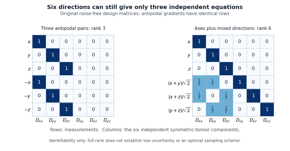
Original design-matrix example: antipodal axes give rank three, while axes and mixed directions give rank six
. Reused algebra illustration, not a reconstruction of a published acquisition or simulation. Rows represent measurements; columns represent the six independent tensor coefficients. Details.Full matrix rank is not a guarantee of a stable estimate in noisy data. If must also be fitted, its logarithm is another unknown; the augmented signal model needs a corresponding independent baseline constraint. The six-coefficient argument above explicitly assumes is separately known. Likewise, tractography requires additional interpretation beyond uniqueness of a local tensor.
A perfect sink condition in drug release is an idealized receiving boundary that removes released drug fast enough for its concentration there to be treated as zero. In diffusion-controlled drug release, this preserves the largest concentration drop available at the exposed boundary. It is a condition on transport at the release surface, rather than a statement that the entire apparatus contains no drug.
For a planar matrix occupying , a common diffusion equation model useswhere is dissolved-drug concentration and is its diffusion coefficient; the outward flux magnitude is used when reporting a positive drug release rate. A finite mass-transfer boundary in drug release instead allows a nonzero surface concentration. If the same concentration scale applies on both sides of the interface, an external transport model iswith transfer coefficient , surface concentration and well-mixed bulk concentration . A small does not force to be small when a stagnant layer or membrane imposes substantial resistance.
An original finite-reservoir example separates capacity from transport. Suppose a formulation can release into , and measured solubility in the chosen medium is . Even after complete release the well-mixed bulk concentration is only . In a simple saturated-interface dissolution model , that concentration still reduces flux to of its zero-bulk-concentration value. Large capacity makes a zero-concentration approximation plausible to a chosen tolerance; it does not make the approximation exact.
A useful experimental test compares in vitro drug release test curves while increasing receiving volume or flow, with temperature and medium chemistry controlled. Sampling and medium replacement require sampling correction in drug release testing. If increasing external transport changes the curve, apparatus resistance or accumulation may still matter. The FDA’s primary account of adaptive perfusion describes pressure-driven filtration designed to avoid rate limitation by a passive dialysis membrane.[ref]
Adaptive Perfusion: A Novel In Vitro Drug Release Testing Method for Complex Drug Products by the FDA. Technology Summary, membrane transport and tangential-flow filtration
The ideal boundary should be distinguished from a method’s practical sink criterion. The FDA’s 1997 dissolution guidance discusses medium, apparatus and agitation together and explicitly allows justified non-sink tests; a zero boundary is a modelling choice to be checked against the actual experiment.[ref]
Dissolution Testing of Immediate Release Solid Oral Dosage Forms by the FDA. Appendix A, pp. A-1–A-2, Dissolution Medium and Agitation
The Higuchi equation models cumulative drug release proportional to the square root of time:Here must be defined: in the planar matrix model it is released mass per exposed area, not the instantaneous drug release rate. The coefficient consequently has units of mass per area per square root of time. Takeru Higuchi’s 1963 primary paper distinguishes drug dispersed in a homogeneous matrix from drug leached from a granular matrix and considers planar and spherical geometries.[ref]
An explicit planar moving-front approximation explains the square root. Let initial total drug loading be per matrix volume, dissolved-drug solubility be , and diffusion coefficient be . Assume excess dispersed solid, rapid local dissolution, an intact non-swelling matrix, constant , a perfect sink condition in drug release and a nearly linear dissolved concentration profile across a depleted layer of depth . The remaining dissolved amount in that layer per area is , so conservation of mass givesCombining and integrating from zero released amount yieldsThis is the quasi-steady front construction; it is not the exact solution for an initially dissolved drug with no excess solid. The profile approximation is most plausible when is large compared with and a substantial undissolved region remains.
For original illustrative values , and , the model gives . At four hours it predicts twice that released amount, not four times. The depleted-layer depth at one hour is approximately . A finite matrix cannot sustain the law indefinitely: once the front approaches the far boundary, the assumed geometry and drug inventory must be reconsidered.
A useful experiment plots corrected released mass per area against and checks whether the apparent slope changes with medium flow or formulation thickness. A straight segment alone does not identify the mechanism. External transport resistance, swelling or changing diffusivity can invalidate the model even if a short data segment looks nearly linear. Sampling correction in drug release testing and a specified exposed area are therefore part of interpreting a fitted .
Here thermal diffusion means the spreading of temperature by thermal conduction. In a stationary homogeneous material with constant thermal conductivity , mass density and specific heat capacity , energy balance and Fourier's law give the heat equation , where is the thermal diffusivity.
Photon diffusion approximates the spreading of radiation after many scattering events have largely randomized propagation directions. Individual photons travel along paths; their distribution can obey a diffusion equation on scales much larger than a transport mean free path. The longer arrival times arise from longer, repeatedly redirected paths.
For homogeneous, conservative isotropic scattering, the photon diffusion coefficient for isotropic scattering is , where is the transport speed and the scattering mean free path. Directional persistence replaces that scale by a transport mean free path in an appropriate transport model. Crossing a characteristic thickness then takes a time of order , with geometry-dependent factors, which can greatly exceed the direct travel time .
A diffuse photon time-of-flight experiment sends a short pulse into a scattering sample and measures the delayed transmitted or returning light. A pulsed source, a fast photodetector and time-correlated single-photon counting can build an arrival-time histogram from repeated pulses. The detector's timing response must be accounted for before attributing all measured broadening to the sample.[ref]
Time-Correlated Single Photon Counting (technical note v. 2.1) by Michael Wahl. Scattering-medium response measurement and iterative reconvolution, p.3
The 1989 study by M. S. Patterson, Britton Chance and B. C. Wilson used a slab diffusion model to relate picosecond-pulse reflectance and transmittance to absorption and scattering, comparing predictions with preliminary measurements and Monte Carlo simulations.[ref]
Time resolved reflectance and transmittance for the non-invasive measurement of tissue optical properties by M. S. Patterson and others. Abstract: model, optical interaction coefficients and experiment/simulation comparison
The earliest nearly unscattered light, nearby boundaries and strongly directional transport can require a fuller radiative transfer description.Restricted diffusion is diffusion whose displacement statistics are constrained by boundaries that particles cannot cross. A reflecting boundary condition models an impermeable wall: particles continue moving, but there is no normal diffusive flux through it. Finite permeability would require a different boundary model.
A physical demonstration uses a liquid confined between solid lamellae. In his first-person account, John E. Tanner described constructing 99 mica layers separated by aluminium-foil strips, removing wrinkles and burrs to obtain regular spacing; Edward O. Stejskal inspected the stack with a stereomicroscope. Pulsed magnetic-field gradients encode displacements in the nuclear magnetic resonance signal, allowing motion normal to the barriers to be compared with less confined directions.[ref]
John Tanner, the return to Germelshausen, and the work that nearly never happened by Derek Jones. Printed p.6, mica-stack account and Figure3
This is a material confinement experiment, not a change in the liquid's chemistry.For an original one-dimensional model, let particles diffuse in with constant diffusion coefficient :The wall conditions are homogeneous Neumann boundary conditions for the diffusion equation. Start in equilibrium, so has the uniform distribution on . Its variance isAt long time separation, the positions decorrelate. Consequently the mean squared displacement approachesAt short times relative to , most displacements have not encountered a wall, and the leading scale is the free-diffusion result . For a hypothetical gap , the long-time plateau is and its root is about .
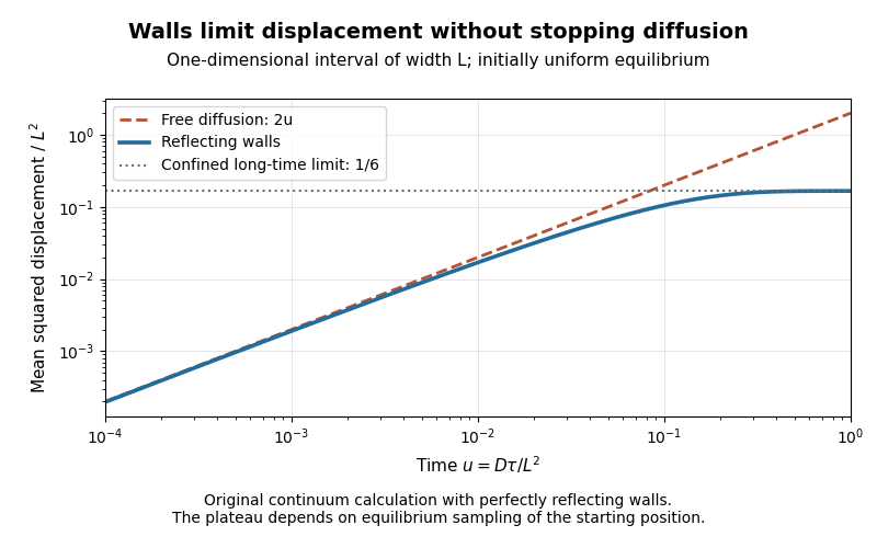
Equilibrium restricted diffusion saturates in a reflecting interval
. Original Neumann-eigenmode calculation with uniform initial positions; time is and mean squared displacement is divided by . Perfectly reflecting walls give a plateau , while free diffusion continues as . These are model curves, not measurements of the mica stack. Details.The initial condition matters: fixing instead gives the long-time value . Likewise, echo attenuation in a confined sample must not automatically be converted into a free-diffusion coefficient. Confinement geometry, timing and the selected boundary model all affect the inference.
A diffusion tensor describes direction-dependent diffusive flux. In the local, linear Fickian model,where is concentration and the entries of have the units of a diffusion coefficient. A scalar coefficient is recovered when . Material models can instead specify a diagonal matrix or symmetric matrix to represent anisotropic transport.[ref]
Diffusion in solids in the COMSOL 6.4 documentation. Solid, Diffusion: isotropic, diagonal and symmetric diffusion coefficients
For an original two-dimensional example, chooseA concentration gradient directed along , with components , produces diffusive flux in consistent units. The flux need not be antiparallel to the gradient. Nevertheless,for every nonzero gradient in this positive-definite matrix example.
The eigenvectors and have eigenvalues 3 and 1. They identify the principal directions and coefficients. Rotating the coordinate basis changes the matrix entries according to ; it does not change these principal coefficients. In an unbounded, homogeneous, drift-free Gaussian model, displacement covariance is , so spreading also differs along those directions.
Symmetry and positive definiteness are assumptions of this ordinary reciprocal diffusion model, not a definition covering every transport law called a tensor. Boundaries also matter: a reflecting boundary condition constrains , which need not be proportional to the normal derivative alone.
The Laplace mechanism releases a numerical query with added Laplace distribution noise scaled to the query's sensitivity. For , define its sensitivity under the chosen dataset adjacency byFor and positive finite sensitivity, release with independent noise coordinates of density , where . The ratio of output densities for adjacent inputs is bounded by , by the triangle inequality. Integrating over any measurable output event proves differential privacy.[ref]
For a count with add/remove sensitivity one and , the noise scale is two and its variance is . Smaller privacy parameters increase uncertainty in this mechanism. A fixed output when sensitivity is zero needs no noise. The adjacency convention is essential: changing what one person can contribute changes the required sensitivity bound.
The epithalamus is a dorsal posterior subdivision of the diencephalon, associated with the roof of the third ventricle. Its usual anatomical scope includes the habenula and associated fiber systems, the pineal gland and the epithelial ventricular roof. It is a region containing distinct structures, not merely another name for the pineal gland.[ref]
Epithalamus in NLM MeSH. Scope note: dorsal posterior position and usual components; classification convention for paraventricular thalamic nuclei.
One component supplies an experimentally clear example. Masayuki Matsumoto and Okihide Hikosaka recorded from the lateral habenula during a reward-associated eye-movement task in rhesus monkeys. Many neurons increased activity for an unrewarded target and decreased activity for a rewarded target, while recorded dopamine-neuron responses showed the opposite pattern.[ref]
Lateral habenula as a source of negative reward signals in dopamine neurons by Masayuki Matsumoto and Okihide Hikosaka. 2007 abstract: visually guided task and opposite reward-related response signs.
Reversing which target location earned reward also reversed the responses. This is an illuminating control: a response following the reward assignment is harder to explain as a fixed preference for one screen position. Habenular excitation preceded dopamine-neuron inhibition on unrewarded trials, and weak electrical stimulation of the lateral habenula inhibited dopamine neurons.[ref]
Lateral habenula as a source of negative reward signals in dopamine neurons by Masayuki Matsumoto and Okihide Hikosaka. Reward-location reversal, temporal order and stimulation results.
Recording and intervention provide different evidence. Opposite responses and timing motivate a circuit hypothesis; stimulation tests influence on another population. Neither establishes that every epithalamic structure performs reward evaluation, nor that the influence is necessarily a direct monosynaptic inhibitory connection. Anatomical membership should not be confused with uniform physiological function.
Pinned article: Introduction to the OurBigBook Project
Welcome to the OurBigBook Project! Our goal is to create the perfect publishing platform for STEM subjects, and get university-level students to write the best free STEM tutorials ever.
Everyone is welcome to create an account and play with the site: ourbigbook.com/go/register. We belive that students themselves can write amazing tutorials, but teachers are welcome too. You can write about anything you want, it doesn't have to be STEM or even educational. Silly test content is very welcome and you won't be penalized in any way. Just keep it legal!
Intro to OurBigBook
. Source. We have two killer features:
- topics: topics group articles by different users with the same title, e.g. here is the topic for the "Fundamental Theorem of Calculus" ourbigbook.com/go/topic/fundamental-theorem-of-calculusArticles of different users are sorted by upvote within each article page. This feature is a bit like:
- a Wikipedia where each user can have their own version of each article
- a Q&A website like Stack Overflow, where multiple people can give their views on a given topic, and the best ones are sorted by upvote. Except you don't need to wait for someone to ask first, and any topic goes, no matter how narrow or broad
This feature makes it possible for readers to find better explanations of any topic created by other writers. And it allows writers to create an explanation in a place that readers might actually find it.
Figure 1. Screenshot of the "Derivative" topic page. View it live at: ourbigbook.com/go/topic/derivativeVideo 2. OurBigBook Web topics demo. Source. - local editing: you can store all your personal knowledge base content locally in a plaintext markup format that can be edited locally and published either:This way you can be sure that even if OurBigBook.com were to go down one day (which we have no plans to do as it is quite cheap to host!), your content will still be perfectly readable as a static site.
- to OurBigBook.com to get awesome multi-user features like topics and likes
- as HTML files to a static website, which you can host yourself for free on many external providers like GitHub Pages, and remain in full control

Figure 2. You can publish local OurBigBook lightweight markup files to either OurBigBook.com or as a static website.
Figure 3. Visual Studio Code extension installation.
Figure 5. . You can also edit articles on the Web editor without installing anything locally. Video 3. Edit locally and publish demo. Source. This shows editing OurBigBook Markup and publishing it using the Visual Studio Code extension. 
- Infinitely deep tables of contents:




All our software is open source and hosted at: github.com/ourbigbook/ourbigbook
Further documentation can be found at: docs.ourbigbook.com
Feel free to reach our to us for any help or suggestions: docs.ourbigbook.com/#contact