A $15M_{\odot }$ star burns core hydrogen chiefly by the CNO cycle for about $10^7$ years. It commonly evolves towards a red supergiant, though winds and mixing alter its track. Core helium burning lasts of order $10^6$ years. Continued contraction then permits carbon, neon, oxygen and silicon burning, producing successively heavier nuclei up to an iron-group core. Neutrino cooling makes the advanced phases much shorter: carbon burning can last thousands of years, while the final burning stages fall to years or days, with substantial model dependence.

An iron-group core cannot gain energy by ordinary fusion into heavier nuclei. Electron captures, photodisintegration and loss of pressure support lead to stellar core collapse. A core-collapse supernova can eject the envelope and leave a neutron star; strong fallback or a failed explosion can instead produce a black hole. The massive-star endpoint involves core collapse, rather than the quiet carbon-oxygen white-dwarf cooling of the two lower-mass examples.

A $5M_{\odot }$ star has a much greater luminosity and exhausts central hydrogen in roughly $10^8$ to $2\times 10^8$ years, mainly through the CNO cycle. It crosses the Hertzsprung gap, develops shell hydrogen burning and ignites core helium without the strongly degenerate helium flash of the solar-mass case. Core helium burning lasts roughly $10^7$ years, with possible blue-loop evolution depending on the model.

It subsequently develops a carbon-oxygen core and double-shell burning on the Asymptotic giant branch, with thermal pulses, winds and envelope loss. For ordinary isolated evolution at this mass, the core does not reach sustained carbon ignition and the final remnant is a carbon-oxygen white dwarf. The broad boundary between white-dwarf and core-collapse outcomes depends on composition, overshooting, rotation and mass loss; the quoted mass is comfortably in the usual intermediate-mass regime.

A $1M_{\odot }$ star spends roughly $10^{10}$ years on the main sequence, deriving most of its luminosity from the proton–proton chain. After central hydrogen depletion, shell hydrogen burning around a contracting helium core expands it into a red giant. The low-mass helium core becomes electron-degenerate before the helium flash. Subsequent core helium burning by the Triple-alpha process, with alpha capture producing oxygen, lasts of order $10^8$ years.

After central helium exhaustion, hydrogen and helium shells burn around a carbon-oxygen core on the Asymptotic giant branch. Strong mass loss removes the envelope, potentially making a planetary nebula, and the remnant becomes a carbon-oxygen white dwarf. It cools using stored thermal energy and does not ignite sustained carbon burning. Detailed durations depend on composition and mass loss; the nuclear endpoint of the isolated solar-mass model is a white dwarf.

Near a red giant's compact core, intense nuclear burning in a small region can produce a large $L_r/m_r$ and a steep required radiative gradient. Where this exceeds the adiabatic gradient, convection transports the released energy and mixes fuel. Core helium burning is a clear example: the strongly temperature-sensitive Triple-alpha process commonly produces a convective burning core; shell flashes can also make convective regions.^[ref]

The qualification matters: an inert degenerate helium core and a steady hydrogen-burning shell on the first-ascent red giant branch are not universally convective; conduction or radiation may dominate there. Red giants also commonly have deep convective envelopes. The physical condition is an excessive required radiative gradient, not proximity to the centre alone.

In the Sun's cool outer layers, partial ionization lowers the adiabatic temperature gradient, while large opacity makes radiative transport inefficient. The required radiative gradientcan exceed ${\nabla }_{\mathrm{ad}}$, so convection carries part of the outward luminosity. The Sun therefore has an outer convective envelope, above its primarily radiative interior. Here $a$ is the radiation constant, $\kappa$ opacity per unit mass and $m_r,L_r$ the enclosed mass and luminosity. Near the visible surface, radiative losses are again important and the flow need not be perfectly adiabatic.

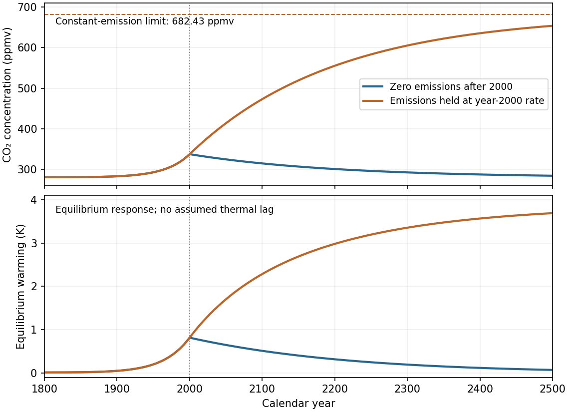
Holding emissions at $E_{00}=8.069\mathrm{GtC}\mathrm{y}{\mathrm{r}}^{-1}$ gives equilibrium concentrationFor time $t$ since 2000,It increases monotonically on the same 200-year timescale and reaches about $654.07\mathrm{ppmv}$ in 2500. The limiting, and hence peak asymptotic, warming isIn 2500 the equilibrium warming is about $3.69\mathrm{K}$, still below that asymptote. A stable thermal adjustment much faster than the carbon timescale follows this slow approach with a short lag and has the same limiting warming. These are predictions of the specified linear reservoir model, not a claim that constant real emissions produce a finite universal atmospheric equilibrium.

Let $t=0$ now denote the year 2000 and $C_{00}=336.95\mathrm{ppmv}$. When emissions stop, the model givesThe concentration peaks at the switch, then returns exponentially to $279\mathrm{ppmv}$; in 2500 it is about $283.76\mathrm{ppmv}$. Before 2000 both scenarios share the exponential-emissions trajectory.

Using the specified logarithmic equilibrium warming relative to $C_0$,gives the fast-adjustment peak estimateAn unspecified finite thermal response time below twenty years delays and reduces that peak relative to the instantaneous-equilibrium value; its exact amount cannot be fixed without a response law and a chosen thermal time. The carbon-removal time is much longer, so the warming subsequently declines gradually in this model. Taking the 1800 concentration $280$ as the temperature reference instead changes the quoted estimate by only $0.016\mathrm{K}$.

For the quadratic Planck function profile,The optically thick limit and the instantaneous doubled-abundance result are thereforeThe new coefficient is $\beta /4$, since $B(\tilde{\tau })=B_0+\beta (\tilde{\tau }/2{)}^2$ at fixed physical temperature. For positive $\beta$, the outgoing spectral irradiance decreases. The factor differs from the linear case because the temperature-dependent source function curves with depth; doubling abundance does not mean holding its old functional coefficients fixed in the new optical-depth coordinate.

For the linear Planck function profile, direct integration givesin the optically thick limit. A sudden doubling of absorber abundance doubles optical depth at every physical height while initially leaving the temperature profile fixed. With $\tilde{\tau }=2\tau$, the same profile is $B=B_0+(\alpha /2)\tilde{\tau }$, not $B_0+\alpha \tilde{\tau }$. ThusIf temperature increases downward, $\alpha >0$ and outgoing spectral irradiance decreases immediately because the effective emitting region moves upward into cooler gas. Subsequent thermal adjustment is outside this instantaneous comparison.

The International Linear Collider uses externally powered superconducting niobium RF cavities at about $1.3$ GHz, with a reference average accelerating gradient of $31.5$ MV/m. Superconducting walls reduce RF dissipation, allowing relatively long RF pulses and bunch trains, at the cost of cryogenic infrastructure.

The Compact Linear Collider uses normal-conducting copper structures at about $12$ GHz and a main-linac gradient near $100$ MV/m in its multi-TeV design. A separate high-current, lower-energy electron drive beam is decelerated in power-extraction structures; the resulting RF power accelerates the high-energy, low-current main beams. This two-beam concept supplies short, high-power pulses without requiring a high-power klystron at every main-beam structure.

ILC: superconducting low-loss RF; CLIC: high-gradient normal-conducting two-beam RF. Both rely on damping and final focusing to obtain very small collision spots, so energy alone does not determine their luminosity. ^{[ref] [ref]}

For a comparison appropriate to this 2012 examination, use the reference-design and conceptual-design targets rather than later revised starting stages:The ILC reference programme included scanning approximately $200$–$500$ GeV and a possible $1$ TeV upgrade. The CLIC 2012 studies included lower-energy construction stages as well as the ultimate multi-TeV machine. These are design goals, not achieved operating luminosities.

Collider luminosity sets the event rate for a process of cross-section $\sigma$ through $dN/dt=\mathcal{L}\sigma$; it is not radiated optical power. ^{[ref] [ref]}

Both machines are proposed electron–positron linear colliders, using sources, damping rings, bunch compressors, two opposing main linacs, and final-focus and beam-delivery sections that bring very small bunches to an interaction point. The spent beams go to extraction lines and beam dumps rather than making repeated collision turns.

In the exam-era International Linear Collider reference design, polarized electrons and an undulator-based positron source feed damping rings and two superconducting main linacs; the full $500$ GeV centre-of-mass facility is about $31$ km long. The Compact Linear Collider adds high-current drive-beam generation and deceleration lines parallel to its main linacs; its $3$ TeV concept is roughly $48$ km long. The linear layout avoids the repeated synchrotron-radiation losses that would be severe for multi-hundred-GeV electrons in a storage ring. ^{[ref] [ref]}

Use a calibrated, nonintercepting DC beam current transformer to measure the circulating current repeatedly during a fill, with top-up injection absent or separately recorded. At fixed revolution frequency, $I=eN{f}_{\mathrm{rev}}$, so a fit to $\log I$ versus time gives slope $-1/\tau$ for exponential decay. The transformer's zero offset and long-term drift must be controlled, especially at low current. An AC current transformer or a calibrated bunch pickup can additionally resolve bunch charge, whereas a DC transformer provides the total circulating intensity needed here.

Particles are lost when a process drives their transverse amplitude or energy outside the machine's accepted region. Principal causes include scattering from residual gas; Touschek scattering within a bunch, which can convert transverse momentum into excessive longitudinal momentum; collision losses at an interaction point; diffusion from nonlinear resonances, field or RF noise; and collective instabilities or insufficient RF acceptance. Mechanical aperture restrictions turn large-amplitude motion into a loss.

Synchrotron-radiation energy loss is normally replenished by RF, so it does not by itself remove one electron for each emitted photon. Rare large energy deviations can nevertheless contribute to losses if they exceed the accepted energy range. Continuous top-up injection can hide the underlying decay and must be accounted for when measuring a lifetime.

The instantaneous beam lifetime iswhere losses make $dN/dt<0$. If the fractional loss rate is constant, $N(t)=N_0{e}^{-t/\tau }$ and $\tau$ is the time to fall to $1/e$ of the starting population. At fixed revolution frequency, the circulating current has the same exponential decay. Density-dependent loss mechanisms can make the instantaneous lifetime vary, so a single exponential need not fit every fill.

The RF harmonic number is the number of RF cycles per revolution, so $f_{\mathrm{RF}}=h{f}_{\mathrm{rev}}$. For $h=32$,The synchronous phase fixes which phase of that voltage is sampled, not the frequency ratio. For a sine voltage, ${\phi }_s=0$ gives zero net accelerating voltage and describes a stationary ideal-energy condition; an actual energy ramp requires a phase producing the required energy gain. A different phase-origin convention changes that statement about the zero of phase, but not the boxed frequencies.

The quoted proton energies are explicitly kinetic. For mean ring radius $\bar{R}=215$ m,Using these expressions rather than setting $\beta =1$ at injection givesThe frequency approaches $c/C$ as energy increases; it is the velocity increase, not a change in the prescribed mean ring circumference, that produces the frequency sweep.

As the star expands onto the red giant branch, a planet of fixed radius produces a shallower exoplanet transit, $\delta \propto R_{\star }^{-2}$. For a fixed circular orbit and an approximately central chord, duration grows approximately as $R_{\star }$, and transit probability also rises. At fixed orbital inclination the impact parameter in stellar-radius units decreases, further changing the chord. These statements neglect orbital evolution, stellar mass loss, tidal effects and eventual engulfment, all of which can matter for a very close planet.

Limb darkening makes the central stellar surface brighter than the disk mean. A small planet at projected position $\mathbf{x}$ blocks fractional flux approximately $\delta (\mathbf{x})=(R_p/R_{\star }{)}^{2}I(\mathbf{x})/⟨I⟩$. A central transit is therefore deepest near mid-transit and rounded rather than flat-bottomed; a near-limb chord can be shallower. The geometrical contact times do not change for fixed radii and orbit, although a threshold-based measured duration can change because ingress and egress are fainter.

Reducing orbital inclination from exactly edge-on increases the impact parameter and shortens the chord, giving $t_{\mathrm{tr}}\propto \sqrt{1-b^2}$ in the small-planet, circular approximation. For a uniformly bright disk, a fully internal transit retains approximately the same exoplanet transit depth $(R_p/R_{\star }{)}^2$. Once grazing, the occulted area and exoplanet transit depth decrease; for $b>1+R_p/R_{\star }$ the exoplanet transit disappears. With limb darkening, a higher-$b$ path is also typically shallower before grazing.