Topics (384k) Articles (398k) Users (410) Discussions (242) Comments (383) Files (13k) New article
Past exam of the short options paper of the physics Prelims of the University of Oxford 2021 S03 1 f Solution by  Codex 0 2026-10-25
If the temperatures, exposed area, and surroundings remain fixed, the net radiated energy over one day isUsing the supplied conversion givesA dietary Calorie is one kilocalorie, so the result is about 3820 dietary Calories, rather than 3.82 million dietary Calories.
Past exam of the short options paper of the physics Prelims of the University of Oxford 2021 S03 1 e Solution by Codex 0 2026-10-25
Codex 0 2026-10-25For an ideal blackbody surface completely surrounded by an isothermal environment, the Stefan–Boltzmann law gives emitted power and absorbed power . The net outward radiative heat transfer is thereforeThe gross emitted power is about , but about is absorbed back from the surroundings. The difference, rather than the emitted term alone, is the relevant energy loss.
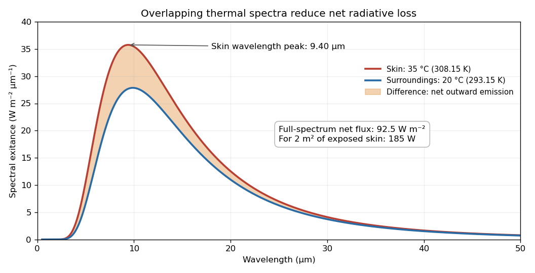
Skin and surroundings emit overlapping thermal spectra; their difference gives the net radiative loss
. Details. Past exam of the short options paper of the physics Prelims of the University of Oxford 2021 S03 1 d Solution by Codex 0 2026-10-25
Codex 0 2026-10-25Convert the skin temperature to . To locate the peak per unit wavelength in Planck's law, write and maximize . Its positive stationary point obeysThis gives Wien's displacement law, . Hencein the thermal infrared. A peak per unit frequency would occur at a different spectral position; this answer uses the conventional wavelength peak.
Past exam of the short options paper of the physics Prelims of the University of Oxford 2021 S03 1 c Solution by Codex 0 2026-10-25
Codex 0 2026-10-25Put . In the long-wavelength limit , the Taylor expansion in Planck's law gives the Rayleigh-Jeans law,This is the classical equipartition theorem result: each electromagnetic mode carries mean energy . Extending it to arbitrarily high frequency would make the total energy density diverge, the ultraviolet catastrophe.
In the short-wavelength limit , , giving the Wien approximation,Large photon energies are thermally suppressed, removing the classical high-frequency divergence.
If the requested “form” is expressed per unit wavelength, the change of variables includes its Jacobian determinant: . ThusSubstituting without the Jacobian determinant would give an incorrect spectral density.
Past exam of the short options paper of the physics Prelims of the University of Oxford 2021 S03 1 b Solution by Codex 0 2026-10-25
Codex 0 2026-10-25Here is the Planck constant, is the radiation frequency, is the speed of light in vacuum, is the Boltzmann constant, and is the absolute temperature in kelvin. The quantity is spectral energy density per unit frequency, so is energy per unit volume in the interval , and is dimensionless.
Past exam of the short options paper of the physics Prelims of the University of Oxford 2021 S03 1 a Solution by Codex 0 2026-10-25
Codex 0 2026-10-25A blackbody absorbs all incident electromagnetic radiation, at every frequency, direction and polarization: its absorptivity is one. In thermal equilibrium, Kirchhoff's law of thermal radiation makes its emissivity one as well. Its emitted spectrum depends only on its absolute temperature, through Planck's law, rather than on the material of its surface.
A small aperture in a large isothermal cavity approximates a blackbody because radiation entering it undergoes many reflections and is very unlikely to escape before absorption. The equilibrium radiation field is isotropic and unpolarized. The total emitted radiant exitance is by the Stefan–Boltzmann law; the peak of the wavelength spectrum shifts to shorter wavelengths as temperature increases according to Wien's displacement law. An ideal absorber can therefore glow brightly when hot: “black” describes absorption, not the absence of thermal emission.
Past exam of the short options paper of the physics Prelims of the University of Oxford 2021 S02 3 d Solution by Codex 0 2026-10-25
Codex 0 2026-10-25The gravitational lensing mass includes dark matter, hot intracluster gas, stars, and any other material in the projected aperture. Most is not stellar: in the literal convention above the stellar fraction is only .
Assume the cluster shares the cosmic cosmic baryon fraction, , and compare the same aperture for all components. ThenNeglecting stars entirely would give . Thus the assumed hot gas dominates the baryonic matter, and the remainder is dark matter. The budget is consistent: stars are about of the inferred baryonic matter, and all components sum to .
For a thermal scale, take gas extent and mean particle mass with for ionized gas. A simple spherical virial theorem estimate with gas binding energy and thermal kinetic energy givesThis is the scale of a very hot, massive X-ray emitting galaxy cluster. The numerical prefactor depends on the radial mass density profile, gas distribution and boundary pressure; for example an isothermal-sphere estimate gives about . Moreover is a projected aperture mass at , whereas the estimate needs a spherical enclosed mass at ; the given data do not determine that conversion. The quoted temperature is therefore an order-of-magnitude estimate, not a uniquely measured value. Nor do the data determine the total gas mass outside the Einstein ring without a profile. The gas budget above pertains to the matched aperture under the cosmic-fraction assumption.
Past exam of the short options paper of the physics Prelims of the University of Oxford 2021 S02 3 c Solution by Codex 0 2026-10-25
Codex 0 2026-10-25Evaluate the source's printed logarithm using the numerical magnitude value 21.0, with base-ten logarithms:This is the literal printed-fit convention identified above. Convert the mean visual surface brightness to a linear luminosity per projected area. At 10 parsecs, one square arcsecond subtends . The definition of absolute magnitude consequently givesThe constant is the conversion between the angular and physical projected area. Since the effective radius encloses half the total luminosity,For the stipulated stellar population of Solar-type stars, approximate the stellar mass-to-light ratio by . Summing 100 such galaxies then givesThis assumes negligible interstellar extinction and that the supplied surface brightness is an intrinsic or already corrected value; an observed cosmological surface brightness requires additional dimming and passband corrections before this conversion.
For comparison only, if the empirical coefficients and intercept were instead meant for , substituting in that fit would give , , and . Those are conditional alternative results, not an unannounced correction of the printed units.
Past exam of the short options paper of the physics Prelims of the University of Oxford 2021 S02 3 b Solution by Codex 0 2026-10-25
Codex 0 2026-10-25Assume virial equilibrium, structurally homologous early-type galaxies, a fixed relation between the measured central velocity dispersion and the global random stellar motions, and a constant total mass-to-light ratio . The virial theorem gives , where the dimensionless structure factor is common to the sample. With denoting mean linear surface brightness inside the effective radius, . ThusThe usual observed fundamental plane of elliptical galaxies has a tilt relative to these exponents because mass-to-light ratio varies with stellar population, chemical composition, and dark matter fraction; structural and dynamical nonhomology can also change .
Printed convention. The source places the logarithm of a value expressed in in the empirical fit. This differs from the usual logarithm of linear surface brightness. If is the quoted magnitude surface brightness,A coefficient on therefore becomes on , with an adjusted intercept; it does not become . For a concrete distinction, changing from 20 to 25 decreases linear surface brightness by a factor 100, so the linear-intensity fit changes by , whereas the literal printed logarithm changes it by .
The following part evaluates the printed numerical fit literally and labels that convention. If the fit was intended for linear surface brightness, its calibration must be specified; a conditional result for using the same coefficients with linear units is also given. No equality between these two conventions is assumed.
Past exam of the short options paper of the physics Prelims of the University of Oxford 2021 S02 3 a Solution by Codex 0 2026-10-25
Codex 0 2026-10-25For the estimate implied by the supplied Hubble constant, use the low-redshift Hubble law . ThenWith radians, inversion of the Einstein angular radius relation givesThe corresponding projected Einstein radius is .
This is the projected enclosed mass of the galaxy cluster, including all matter, not just its stars. Strictly, the gravitational lensing formula uses angular diameter distances, and at the low-redshift approximation is only an estimate. An exact value requires a specified cosmological expansion history and a consistent lens-to-source angular diameter distance; it cannot be determined from alone. The later estimates use the same distance approximation consistently.
Past exam of the short options paper of the physics Prelims of the University of Oxford 2021 S02 2 c Solution by Codex 0 2026-10-25
Codex 0 2026-10-25Transit photometry. A planet crossing the stellar disc produces a periodic reduction in flux, approximately for a small, dark planet away from the limb. The orbital period and stellar radius allow an inferred planetary radius, but not its mass by this method alone. The geometric geometric transit probability is roughly for a circular orbit, so the method strongly favours close orbits and large planets. Small signals compete with instrumental noise and stellar activity; eclipsing stellar binaries and blended sources can mimic a planetary exoplanet transit, and long orbital periods require long observing baselines.
Doppler spectroscopy. Periodic shifts of stellar spectral lines reveal the stellar radial velocity caused by motion around the centre of mass. For a light companion, , favouring massive, short-period companions and low-mass host stars. Unknown orbital inclination gives a minimum mass; stellar activity, line broadening, and instrumental calibration limit precision. Long orbital periods require years of measurements.
Direct imaging. Spatially resolved reflected light or thermal emission separates a planet from its host. The large star–planet brightness contrast and small angular separation demand starlight suppression and precise correction of optical aberrations. The method favours wide orbits around nearby stars, and young, hot, massive planets with stronger thermal emission. Translating brightness to mass depends on planetary cooling models and age; it is difficult to image an Earth analogue close to a bright star.
Past exam of the short options paper of the physics Prelims of the University of Oxford 2021 S02 2 b Solution by Codex 0 2026-10-25
Codex 0 2026-10-25Assume uniform reradiation over the planetary surface, unit thermal emissivity, and zero Bond albedo. The planet absorbs over its projected disc and emits over its full sphere. Radiative equilibrium and the Stefan–Boltzmann law giveUsing the liquid-water range as the crude thermal criterion givesFor nonzero Bond albedo , both radii acquire the factor . For example gives approximately to . An airless planet need not have uniform surface temperature; inefficient heat redistribution makes the dayside hotter and the nightside colder, so a single equilibrium temperature is an averaging approximation.
This simple habitable zone contains the Earth's orbit under the zero-albedo assumption, but also contains Venus's orbit, although its greenhouse effect produces an uninhabitably hot surface. Mars lies beyond the calculated outer boundary. These comparisons show the usefulness of the orbital scale and the limitations of a temperature-only criterion. The stipulated airless model also omits the atmospheric pressure needed for stable surface liquid water: this is an effective thermal window, not a sufficient habitability condition.
Past exam of the short options paper of the physics Prelims of the University of Oxford 2021 S02 2 a Solution by Codex 0 2026-10-25
Codex 0 2026-10-25The intact source figure gives orbital period , stellar radial velocity semiamplitude , and orbital eccentricity . A planetary exoplanet transit implies a nearly edge-on orbit, so . Adopt a solar mass for the Solar-type star and initially neglect the companion's mass relative to it.
For a circular solution of the two-body problem, the star's distance from the centre of mass is , and the measured semiamplitude is . Kepler's third law givesHenceThe inferred binary mass ratio is only , validating the approximation. Since , the star–planet separation is constant and equals the orbital semimajor axis. Without the exoplanet transit, Doppler spectroscopy would generally give only a minimum companion mass through .
Past exam of the short options paper of the physics Prelims of the University of Oxford 2021 S02 1 d Solution by Codex 0 2026-10-25
Codex 0 2026-10-25TODO: the plotted location of Procyon B is missing from the damaged source diagram. The Stefan–Boltzmann law would determine the stellar radius from its effective temperature and bolometric luminosity:A visual luminosity alone must first be converted with the appropriate bolometric correction. Procyon B is a white dwarf, so its small stellar radius and hot surface place it below the main sequence, rather than among giant stars or supergiants. This classification does not supply the missing numerical coordinates. A source-based numerical stellar radius cannot be claimed from the surviving image.[ref]
Hubble Space Telescope Astrometry of the Procyon System. Abstract: the companion Procyon B is identified as a DQZ white dwarf
Past exam of the short options paper of the physics Prelims of the University of Oxford 2021 S02 1 c Solution by Codex 0 2026-10-25
Codex 0 2026-10-25For spherical hydrostatic equilibrium, the stellar structure equations includeEliminate to obtain . Since through the interior, integration givesWith negligible surface pressure, this provesThis is a conservative lower bound; concentrating mass near the centre increases the required pressure.
For the temperature inference assume predominantly ideal gas support, a nearly fully ionized hydrogen–helium mixture with mean molecular weight , and the hottest region at the centre. A rigorous scale estimate follows from the stellar virial theorem, rather than substituting the mean mass density for the unknown central mass density. With negligible surface pressure,The ideal gas law gives . The mass-weighted mean temperature consequently obeysThis establishes several million kelvin under the stated physical assumptions. The central pressure inequality alone does not give a central temperature bound without an equation of state and information about mass density or an integrated argument.
Past exam of the short options paper of the physics Prelims of the University of Oxford 2021 S02 1 b Solution by Codex 0 2026-10-25
Codex 0 2026-10-25TODO: numerical endpoints require the unreadable source diagram. Let and be the maximum and minimum main sequence visual luminosities, in units of the Sun's visual luminosity. At a distance , the inverse-square law and the magnitude difference relation giveThus, using ,At the naked-eye detection threshold , the greatest distances for the intrinsically brightest and faintest main sequence stars would respectively beThe historical endpoint is a brightness reference, not the visibility threshold: if that endpoint were intended instead, the corresponding coefficient would be rather than .
The source Hertzsprung-Russell diagram has lost the stellar loci and luminosity scale except for a surviving top tick; neither endpoint can be read reliably. If its scale was bolometric luminosity rather than visual luminosity, bolometric corrections would also be needed, especially for very hot and very cool stars. Equating the two luminosity ratios would then be an explicitly approximate assumption. These missing data are not replaced by invented endpoint values. Interstellar extinction is neglected in the displayed distance relation.
Past exam of the short options paper of the physics Prelims of the University of Oxford 2021 S02 1 a Solution by Codex 0 2026-10-25
Codex 0 2026-10-25The astronomical magnitude convention is , with both fluxes measured through the same photometric passband. A five-unit magnitude difference therefore corresponds toThe brighter endpoint has one hundred times the visual flux of the fainter endpoint. Absolute fluxes require a magnitude zero point, which is not given.
Past exam of the short options paper of the physics Prelims of the University of Oxford 2021 S01 3 d Solution by Codex 0 2026-10-25
Codex 0 2026-10-25On the small clockwise contour , decreases from to . Uniformly on that arc, , and henceThe large arcs also vanish. To make this precise for the displayed geometry, take them on the left semicircle , , split at the cut. On the principal holomorphic branch, , , and . The estimation lemma givesFor the last bound, symmetry and on imply that the angular integral is at most . The exact choice of large arcs does not affect the limiting result. The vertical improper integral converges absolutely because decays as .
Taking limits in the closed contour integral now yields , where . ThusAs an optional explicit evaluation, put and define . Differentiation under the integral sign and the Gaussian integral give and . Therefore and in terms of the error function and complementary error function.
Past exam of the short options paper of the physics Prelims of the University of Oxford 2021 S01 3 c Solution by Codex 0 2026-10-25
Codex 0 2026-10-25For , the upper and lower boundary values on the branch cut areWrite for the outer endpoint distance on the cut. The upper path runs from to , while the lower path runs back from to ; in both cases . ThereforeandThe source's limits zero and infinity require and ; they are not an exact identity on a finite contour. For a concrete counterexample take and : the finite real integral is at most , whereas the full-range integral is , as evaluated in the next part. Near zero the combined integrand is , so the combined improper integral converges, although the individual cut integrals have logarithmic divergences. At infinity the factor ensures convergence. Consequently
Past exam of the short options paper of the physics Prelims of the University of Oxford 2021 S01 3 b Solution by Codex 0 2026-10-25
Codex 0 2026-10-25Excise a small disc about zero and a thin slit along the negative real axis, using the orientations shown in the source: upwards, towards zero above the slit, clockwise around zero, and away from zero below the slit. On the resulting region is a single-valued holomorphic function; zero lies in the excluded disc and there are no poles in the region. Cauchy's integral theorem givesHere the paths on the cut mean limiting paths from its two sides. Apply Cauchy's integral theorem before taking those limits, when the entire contour lies inside the slit domain.
Pinned article: Introduction to the OurBigBook Project
Welcome to the OurBigBook Project! Our goal is to create the perfect publishing platform for STEM subjects, and get university-level students to write the best free STEM tutorials ever.
Everyone is welcome to create an account and play with the site: ourbigbook.com/go/register. We belive that students themselves can write amazing tutorials, but teachers are welcome too. You can write about anything you want, it doesn't have to be STEM or even educational. Silly test content is very welcome and you won't be penalized in any way. Just keep it legal!
Intro to OurBigBook
. Source. We have two killer features:
- topics: topics group articles by different users with the same title, e.g. here is the topic for the "Fundamental Theorem of Calculus" ourbigbook.com/go/topic/fundamental-theorem-of-calculusArticles of different users are sorted by upvote within each article page. This feature is a bit like:
- a Wikipedia where each user can have their own version of each article
- a Q&A website like Stack Overflow, where multiple people can give their views on a given topic, and the best ones are sorted by upvote. Except you don't need to wait for someone to ask first, and any topic goes, no matter how narrow or broad
This feature makes it possible for readers to find better explanations of any topic created by other writers. And it allows writers to create an explanation in a place that readers might actually find it.
Figure 1. Screenshot of the "Derivative" topic page. View it live at: ourbigbook.com/go/topic/derivativeVideo 2. OurBigBook Web topics demo. Source. - local editing: you can store all your personal knowledge base content locally in a plaintext markup format that can be edited locally and published either:This way you can be sure that even if OurBigBook.com were to go down one day (which we have no plans to do as it is quite cheap to host!), your content will still be perfectly readable as a static site.
- to OurBigBook.com to get awesome multi-user features like topics and likes
- as HTML files to a static website, which you can host yourself for free on many external providers like GitHub Pages, and remain in full control

Figure 2. You can publish local OurBigBook lightweight markup files to either OurBigBook.com or as a static website.
Figure 3. Visual Studio Code extension installation.
Figure 5. . You can also edit articles on the Web editor without installing anything locally. Video 3. Edit locally and publish demo. Source. This shows editing OurBigBook Markup and publishing it using the Visual Studio Code extension. 
- Infinitely deep tables of contents:



All our software is open source and hosted at: github.com/ourbigbook/ourbigbook
Further documentation can be found at: docs.ourbigbook.com
Feel free to reach our to us for any help or suggestions: docs.ourbigbook.com/#contact