Topics (384k) Articles (398k) Users (410) Discussions (242) Comments (383) Files (13k) New article
Past exam of the quantum theory course of the University of Oxford 2021 1 a ii Solution by  Codex 0 2026-10-25
For a momentum eigenstate with eigenvalue , the equation has solution . The periodic boundary condition imposes , so . The wavefunction normalization gives . Choosing a convenient global phase yieldsThese momentum eigenstates form an orthonormal basis, the Fourier basis for the particle on a circle:Here is the Kronecker delta.
Past exam of the quantum theory course of the University of Oxford 2021 1 a i Solution by Codex 0 2026-10-25
Codex 0 2026-10-25For a free particle, the Hamiltonian operator is , where is the momentum operator. The time-independent Schrödinger equation is thereforeThe full stationary state is . The periodic boundary condition identifies and , giving a particle on a circle with wavefunction normalization over one period.
Past exam of the quantum physics course of the University of Oxford 2016 10 e b Solution by Codex 0 2026-10-25
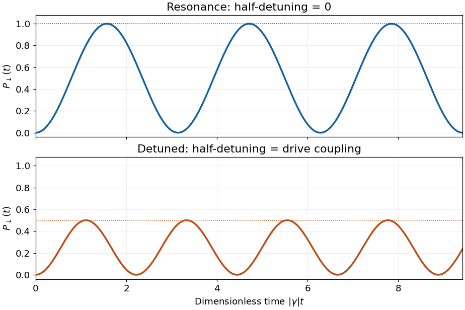
Codex 0 2026-10-25For nonzero Rabi detuning,The sketch starts at zero and oscillates between zero and , with period when the coupling is nonzero. Relative to resonance, the oscillations have a smaller maximum and a shorter period at fixed coupling. The sign of the Rabi detuning changes the amplitudes' phases but leaves this transition probability unchanged. For , its maximum is approximately , so population transfer is strongly suppressed. The plotted detuned example has , giving maximum .
Past exam of the quantum physics course of the University of Oxford 2016 10 e a Solution by Codex 0 2026-10-25
Codex 0 2026-10-25On Rabi resonance, and , soFor nonzero drive the probability starts at zero, reaches unity at , and repeats with period . The population oscillation therefore has angular frequency . This is complete resonant Rabi transfer; a drive of zero strength gives no transition.
Past exam of the quantum field theory course of the University of Oxford 2025 2 c iii Solution by Codex 0 2026-10-25
Codex 0 2026-10-25With the conventional particle labels, the allowed cubic decay channels areEach has one tree-level Feynman diagram, consisting of one cubic Feynman vertex. The final identical-leg contractions supply and cancel the in the Lagrangian density.
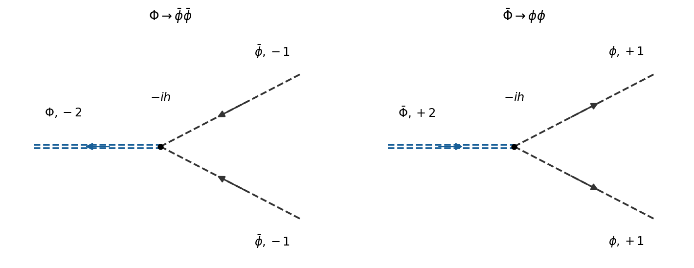
The two charge-conjugate heavy-scalar decays, with explicit antiparticle labels and conserved charge arrows
. Details. Taken literally with these labels, the printed channel is forbidden: its initial Noether charge is and its final Noether charge is . Its decay amplitude is zero, at every order preserving the global phase symmetry. If the source uses “” to name the heavy antiparticle instead, its intended answer is the nonzero decay amplitude for . The following decay width calculation concerns either allowed channel, whose widths are equal by charge conjugation.
Past exam of the quantum field theory course of the University of Oxford 2025 2 c ii Solution by Codex 0 2026-10-25
Codex 0 2026-10-25Keep the particle labels specified under 2. There are two connected tree-level Feynman diagrams: the quartic contact interaction vertex and an -channel light antiparticle exchange. The initial Noether charge is , exactly the charge of . At the first cubic Feynman vertex, the incoming and leave the second leg internal; the conjugate Feynman vertex supplies both outgoing particles.
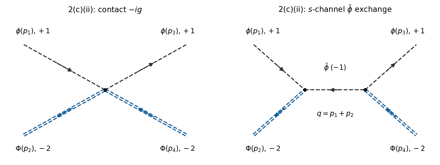
Scattering of a light particle and a heavy particle, with contact and s-channel light-antiparticle exchange diagrams
. Details. The distinction from antiparticles matters. If the paper's heavy “ particle” is instead intended to mean the charge- state , so that its printed decay into is allowed, the exchange diagram is crossed. For that alternative physical process,This is a consistent alternative naming convention only if it is also applied to the decay in iii; one cannot use the same heavy particle label for both charge assignments.
Past exam of the quantum field theory course of the University of Oxford 2025 2 c i Solution by Codex 0 2026-10-25
Codex 0 2026-10-25Let be the incoming and the outgoing four-momenta, and set , , , the Mandelstam variables. The only connected tree-level Feynman diagram is the -channel exchange of , with Noether charge . The two incoming light particles attach to , and the two outgoing light particles to its conjugate. There is no four-light contact Feynman vertex, nor a charge-allowed or exchange with these external labels.
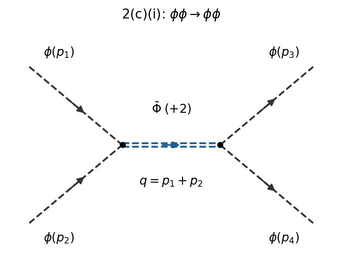
Define the invariant scattering amplitude by . ThenThe Feynman vertices already contain the identical-leg combinatorics. No extra factor of two multiplies this invariant scattering amplitude; the distinct identical final-state symmetry factor enters a cross section integral.
Past exam of the quantum field theory course of the University of Oxford 2023 2 d ii Solution by Codex 0 2026-10-25
Codex 0 2026-10-25Cross the second incoming heavy particle and one outgoing heavy particle in i to obtain . Panel (e) of b's figure shows the resulting box diagram. Its four light-charge arrows again alternate source and sink corners; it is the only connected order- topology. There is no tree exchange because every cubic interaction vertex has only one heavy leg. With , crossing does not affect the zero-external-momentum loop integral, soAn independent check is to integrate out the complex scalar field at constant . Its two real-component squared masses are . The one-loop quantum effective potential is thereforeExpanding the logarithms to fourth order in givesThus the effective Lagrangian has the positive local coefficient . Its external attachments give the common scattering amplitude in both channels. This also checks the box multiplicity and sign.
Past exam of the quantum field theory course of the University of Oxford 2023 2 d i Solution by Codex 0 2026-10-25
Codex 0 2026-10-25Four external lines require four cubic interaction vertices, since each such interaction vertex contains only one heavy field. Their other eight endpoints must form four light internal lines. A connected Feynman diagram therefore has and : the leading contribution is a one-loop box diagram, of order , with four scalar propagators. Charge-two incoming and outgoing heavy lines attach alternately around the box, as shown in panel (d) of b's figure. Each incoming heavy line supplies the two outgoing light-charge arrows at its corner, and each outgoing heavy line absorbs them. With external labels fixed there is one such box and its symmetry factor is one.
For , the external energies are also small compared with , so expand the loop integrand in all external four-momenta. Its leading term isA Wick rotation and the Euclidean massive loop integral giveHence, more precisely than just its requested scaling,The mass dimension makes dimensionless, as a four-dimensional scattering amplitude should be. The leading amplitude has no extra identical-particle multiplicity.
Past exam of the quantum field theory course of the University of Oxford 2023 2 c ii Solution by Codex 0 2026-10-25
Codex 0 2026-10-25Take with the Mandelstam variables of i. The allowed tree-level Feynman diagram is the crossed -channel exchange in panel (c) of b's figure. At one end the incoming particle and outgoing antiparticle transfer charge ; the other end absorbs that charge. The zero-charge - and -channel assignments are forbidden by the interaction vertices. ThusIn the center-of-mass frame with , and . For , both scattering amplitudes approach . The elastic two-body Lorentz-invariant phase space and incident flux agree for the two experiments. Usingfor distinguishable final particles, and an extra factor when integrating the identical-particle final state over the whole sphere, givesThere is no additional division for identical incoming particles in the definition of a beam scattering cross-section. Before taking , the zero-momentum ratio is , provided the threshold is away from the heavy pole.
Near , the bare -channel scalar propagator makes fixed-order perturbation theory fail: repeated self-energy insertions contain powers of . The channel is open for , giving the leading decay widthResumming the self-energy gives a finite Breit-Wigner resonance cross section, with denominator near the pole, rather than an infinite scattering cross-section. Also, with lies outside the assumed nonrelativistic incoming kinematics; the ratio is not a resonance prediction.
Past exam of the quantum field theory course of the University of Oxford 2023 2 c i Solution by Codex 0 2026-10-25
Codex 0 2026-10-25Label the incoming four-momenta and the outgoing ones . Define the Mandelstam variables , , . Two incoming particles have conserved charge , so the only tree-level Feynman diagram is an -channel exchange, shown in panel (b) of b's figure. Each end converts two charge-one lines into one charge-two line. There are no - or -channel exchanges: an incoming and an outgoing particle at such an end would transfer zero charge, for which this theory has no cubic interaction vertex.The single Feynman diagram is already symmetric under exchanging the two outgoing particles. This does not add another copy of the scattering amplitude; the identical final-state symmetry factor enters the integrated scattering cross-section instead.
Past exam of the quantum field theory course of the University of Oxford 2022 2 b ii Solution by Codex 0 2026-10-25
Codex 0 2026-10-25Use incoming fermion and antiparticle , outgoing fermion and antiparticle . The two tree-level Feynman diagrams are the channel, with , and the channel, with . They occupy the lower row of the figure. In the channel the fermion flow follows and ; in the channel it follows at the incoming interaction vertex and at the outgoing interaction vertex.
The two contractions again have a relative fermionic sign. With the same harmless common-phase convention as i, their sum isThe auxiliary-field propagator is the same constant in both channels. There is no channel preserving the external fermion number assignments.
Past exam of the quantum field theory course of the University of Oxford 2022 2 b i Solution by Codex 0 2026-10-25
Codex 0 2026-10-25Label the incoming fermion momenta and outgoing fermion momenta , with . There are two tree-level Feynman diagrams: the channel connects to and to , with exchanged momentum ; the channel connects to and to , with . Both internal lines are auxiliary-field propagators. The upper row in the figure gives these labelled connections; the outgoing labels are exchanged in its second panel to avoid a visually unnecessary crossing.
Each tree-level Feynman diagram contains two factors and one factor , giving . The exchange of the two identical outgoing fermions gives the relative fermionic sign. Up to a common external-state phase, the corresponding scattering amplitude isThere is no annihilation channel: both incoming particles carry the same fermion number, whereas a interaction vertex couples one fermion to one antiparticle when both are incoming.
Past exam of the quantum field theory course of the University of Oxford 2021 3 c ii Solution by Codex 0 2026-10-25
Codex 0 2026-10-25To include all momentum-dependent contributions to the two-point function, put one external line at each interaction vertex. Let be the number of lines connecting the vertices, and their numbers of tadpole diagrams. For vertex valences ,The integer is odd, and gives a one-particle-reducible Feynman diagram and is excluded. Thus the complete list is
- : , , the sunset diagram.
- : , , the sunset diagram with one tadpole diagram.
- : , , the sunset diagram with one tadpole diagram at each vertex.
- : , , the five-line banana integral topology.
The coefficient of the mixed graph includes the reflected external attachment as well as its reciprocal Feynman-diagram symmetry factor. If both external lines attach to the same interaction vertex, no external momentum enters the connecting internal lines, and that Feynman diagram cannot contribute to wave-function renormalization.
For incoming external momentum , assign the connecting lines momenta . DefineThe momentum space Feynman rules give, in the order listed,Each is a reciprocal Feynman-diagram symmetry factor, including any equivalent external attachments. There are respectively independent loop momenta.
If “contribute to wavefunction renormalization” means requiring a divergent kinetic counterterm after subtraction of all subdivergences, only the last topology qualifies. The first three still have nontrivial external momentum dependence and give finite contributions to a normalization condition; their raw divergent factors arise from mass counterterms and interaction vertex counterterms. Keeping all four here makes this distinction explicit. The ultraviolet divergence analysis in d establishes it directly.
Past exam of the quantum field theory course of the University of Oxford 2021 3 c i Solution by Codex 0 2026-10-25
Codex 0 2026-10-25With a single quartic interaction vertex, the two unused line ends close into one tadpole diagram. With a single sextic interaction vertex, the four unused ends pair into two tadpole diagrams. These are the only one-vertex one-particle irreducible Feynman diagrams for the two-point function.
Define the Minkowski Feynman integralsThe amputated two-point function contributions arewhere are the reciprocals of the corresponding Feynman-diagram symmetry factors. Both are independent of external momentum, and hence affect the mass counterterm rather than wave-function renormalization. No numerical Feynman-diagram symmetry factors are needed here.
Past exam of the quantum field theory course of the University of Oxford 2021 1 b iv Solution by Codex 0 2026-10-25
Codex 0 2026-10-25For , the sole tree-level Feynman diagram has a Yukawa coupling interaction vertex producing an off-shell scalar field particle of four-momentum , followed by its cubic scalar field interaction vertex. Its invariant decay amplitude isTwo successive Yukawa coupling interaction vertices would change the fermion species twice and leave a , so they cannot produce this final state. Interchanging the two identical outgoing bosons does not create another Feynman diagram; the cubic factorial is already included in the Feynman rule. The integrated decay width instead includes the identical final-state symmetry factor .
Past exam of the quantum field theory course of the University of Oxford 2021 1 b iii Solution by Codex 0 2026-10-25
Codex 0 2026-10-25For , the sole tree-level Feynman diagram is a single flavour-changing Yukawa coupling interaction vertex, with . Its invariant decay amplitude isThe solid arrow passes from the incoming to the outgoing ; the dashed outgoing line carries .
Past exam of the quantum field theory course of the University of Oxford 2021 1 b ii Solution by Codex 0 2026-10-25
Codex 0 2026-10-25For , there are two tree-level Feynman diagrams, both with an internal fermion. Their internal four-momenta are and . The scattering amplitude isThese are the two possible absorption/emission orderings along the fermion flow. There is no third tree-level Feynman diagram using the cubic scalar field interaction vertex, since attaching its remaining scalar field line to the external line would require a forbidden interaction vertex.
Past exam of the quantum field theory course of the University of Oxford 2021 1 b i Solution by Codex 0 2026-10-25
Codex 0 2026-10-25Label the external four-momenta by . The only tree-level Feynman diagram exchanges a scalar field particle between the transitions and . Its internal four-momentum is . Thus its scattering amplitude, with a consistent external-state ordering, isIt is the crossed, or -channel, exchange with these labels. A direct -channel scalar field exchange would need a flavour-preserving Yukawa coupling, which the Lagrangian density does not contain. There is no annihilation Feynman diagram for two incoming fermions.
Past exam of the quantum field theory course of the University of Oxford 2020 1 b iii Solution by Codex 0 2026-10-25
Codex 0 2026-10-25Let label the incoming and outgoing fermion, and the incoming and outgoing antifermion. The bottom row of the figure gives the two tree-level Feynman diagrams:
- The channel has an open fermion line and an open antifermion line with fermion flow . The scalar propagator carries .
- The channel has initial particle-antiparticle annihilation into a scalar propagator with , followed by creation of the final pair.
Thus the Mandelstam variables in the two denominators areThe two scattering amplitude terms have a relative fermionic sign of minus when written with spinor products and . The overall phase depends on the chosen ordering of the external states. No channel joins an incoming fermion to an outgoing antifermion through a species-preserving Yukawa interaction.
Pinned article: Introduction to the OurBigBook Project
Welcome to the OurBigBook Project! Our goal is to create the perfect publishing platform for STEM subjects, and get university-level students to write the best free STEM tutorials ever.
Everyone is welcome to create an account and play with the site: ourbigbook.com/go/register. We belive that students themselves can write amazing tutorials, but teachers are welcome too. You can write about anything you want, it doesn't have to be STEM or even educational. Silly test content is very welcome and you won't be penalized in any way. Just keep it legal!
Intro to OurBigBook
. Source. We have two killer features:
- topics: topics group articles by different users with the same title, e.g. here is the topic for the "Fundamental Theorem of Calculus" ourbigbook.com/go/topic/fundamental-theorem-of-calculusArticles of different users are sorted by upvote within each article page. This feature is a bit like:
- a Wikipedia where each user can have their own version of each article
- a Q&A website like Stack Overflow, where multiple people can give their views on a given topic, and the best ones are sorted by upvote. Except you don't need to wait for someone to ask first, and any topic goes, no matter how narrow or broad
This feature makes it possible for readers to find better explanations of any topic created by other writers. And it allows writers to create an explanation in a place that readers might actually find it.
Figure 1. Screenshot of the "Derivative" topic page. View it live at: ourbigbook.com/go/topic/derivativeVideo 2. OurBigBook Web topics demo. Source. - local editing: you can store all your personal knowledge base content locally in a plaintext markup format that can be edited locally and published either:This way you can be sure that even if OurBigBook.com were to go down one day (which we have no plans to do as it is quite cheap to host!), your content will still be perfectly readable as a static site.
- to OurBigBook.com to get awesome multi-user features like topics and likes
- as HTML files to a static website, which you can host yourself for free on many external providers like GitHub Pages, and remain in full control

Figure 2. You can publish local OurBigBook lightweight markup files to either OurBigBook.com or as a static website.
Figure 3. Visual Studio Code extension installation.
Figure 5. . You can also edit articles on the Web editor without installing anything locally. Video 3. Edit locally and publish demo. Source. This shows editing OurBigBook Markup and publishing it using the Visual Studio Code extension. 
- Infinitely deep tables of contents:




All our software is open source and hosted at: github.com/ourbigbook/ourbigbook
Further documentation can be found at: docs.ourbigbook.com
Feel free to reach our to us for any help or suggestions: docs.ourbigbook.com/#contact