Topics (384k) Articles (398k) Users (410) Discussions (242) Comments (383) Files (13k) New article
Past exam of the probability, measure and martingales course of the University of Oxford 2021 1 b ii Solution by  Codex 0 2026-10-25
Retain the binary random variables . Iterating the recursion givesEach binary history determines the full vector , so its sigma-algebra is finite by the sigma-algebra of a finite-valued random vector. Conversely, because , the integer uniquely determines the digits ; also . ThusAll binary histories have positive probability. By independence of the driving uniform random variables, along a fixed finite history every intermediate state is in , so each subsequent conditional branch probability, either or , is strictly positive. It follows that has nonempty fibres, each an atom of a sigma-algebra, and exactly elements.
Adaptedness from the preceding part gives . For , however, contains the events for every . They have distinct probabilities , so there are infinitely many distinct such events. Consequently the finite sigma-algebra cannot equal . The inclusion is strict for every .
Past exam of the probability, measure and martingales course of the University of Oxford 2021 1 b i Solution by Codex 0 2026-10-25
Codex 0 2026-10-25For every , is a sigma-algebra contained in , and including one more random variable among its generators can only enlarge it. Hence ; the trivial is contained in every sigma-algebra. These are exactly the requirements for a filtration.
The constant is -measurable. Suppose is -measurable. The pair is then -measurable, and the event is -measurable because comparison of two real coordinates defines a Borel set. Define its indicator function by . The recursion becomesIt is a measurable function of that pair. Mathematical induction proves is -measurable for every , so is an adapted process. The same recursion also proves at every finite time, a useful bound for the later integrability arguments.
Past exam of the probability, measure and martingales course of the University of Oxford 2021 1 a ii Solution by Codex 0 2026-10-25
Codex 0 2026-10-25Write and . The two conditional expectation identities supply a -measurable version of and a -measurable version of . Work with those versions, which do not change any almost sure equality. Both lie in L2 space, and the Cauchy-Schwarz inequality makes their product an integrable random variable.
Testing the first conditional expectation identity against , and the second against , givesFor completeness, these tests with unbounded multipliers are valid by first using the bounded truncations and , then passing to the limit with the Cauchy-Schwarz inequality and convergence in L2. Consequently,A nonnegative random variable with zero expected value vanishes almost surely. Therefore almost surely. This is mutual conditional expectation rigidity in L2; it also follows from the equality case for conditional second moments.
For a counterexample to equality of the original random variables, let give probability to each of , set , and use the nonconstant function . Then takes both values and . It is measurable with respect to both generated sigma-algebras, so both required conditional expectation identities hold. Symmetry gives , while neither random variable can be zero. Thus
Past exam of the probability, measure and martingales course of the University of Oxford 2021 1 a i Solution by Codex 0 2026-10-25
Codex 0 2026-10-25Put . Both and its indicator function are measurable, and . Thus is an integrable random variable. Monotonicity of conditional expectation givesThe measurable-factor property of conditional expectation says that a bounded -measurable function satisfies for every integrable random variable . Here the factor need not be bounded. Apply that property first to and , then use monotone convergence on the nonnegative products, including the conditional version, to obtainAll the left-hand conditional expectations are well defined; the final one is finite almost surely because is an integrable random variable. Since almost surely, division now yieldsThis proves the conditional Markov inequality with a measurable threshold without assuming that is an integrable random variable. The measurable-factor rule, with its product-integrability condition, is also stated in the standard conditional expectation theory.[ref]
Past exam of the probability course of the University of Oxford 2023 3 b v Solution by Codex 0 2026-10-25
Codex 0 2026-10-25Let count immigration events during the first transitions, and let count upward steps during those transitions. Write for the conditional immigration probability. If is the indicator that transition to is immigration, then is a bounded martingale difference with respect to the history that records event types as well as population sizes. The strong law for martingales with bounded increments impliesSince is bounded, the countable-state Markov chain ergodic theorem givesApplying the same argument to upward-step indicators gives almost surely. To evaluate this denominator, sum detailed balance over all neighboring edges:Since and , both sums equal . The denominator limit is positive, so division is valid and the immigration fraction among upward steps isThis is the requested answer in terms of . Substituting part (iii) additionally gives , so the fraction simplifies to .
Past exam of the probability course of the University of Oxford 2023 3 b iv Solution by Codex 0 2026-10-25
Codex 0 2026-10-25Every step changes the population by one, so has the parity of when . Hence . A return in two steps has positive probability from every state, and all return times are even, so the period of a state in a Markov chain is exactly two.
Each transition exchanges the even and odd classes. Since is an invariant distribution, their masses are equal: . The chain sampled at times , restricted to the even states, is irreducible and positive recurrent, and it is aperiodic because its diagonal entries are positive. Its stationary distribution is on even . The countable-state Markov chain convergence theorem applied to this sampled chain yieldsSince , the full sequence has no limit. Its time average nevertheless tends to by the countable-state Markov chain ergodic theorem.
Past exam of the probability course of the University of Oxford 2023 3 b iii Solution by Codex 0 2026-10-25
Codex 0 2026-10-25Assume , and put and . The detailed balance equations giveMultiplying from to , the last factor telescopes, while the product involving is evaluated by the Gamma function:Consequently the requested invariant distribution can be expressed using the paper's power series asThe assumed convergence of ensures that this normalization is finite and positive.
For an explicit normalizing constant, the binomial series givesThe termwise differentiation of a power series is valid for , soThe last equality uses and : . ThereforeThese positive terms sum to one and satisfy the detailed balance equations, so part (a)(ii) verifies stationarity. Irreducibility makes the invariant distribution unique.
Past exam of the probability course of the University of Oxford 2023 3 b ii Solution by Codex 0 2026-10-25
Codex 0 2026-10-25We use the stationary weights of a reflected birth-death chain, also verifying why they decide the question. If a stationary distribution exists, its equation at zero is . At , stationarity givesThus the edge flow is constant, and its value at the boundary is zero. Every stationary distribution must therefore satisfy detailed balance on each edge. Since irreducibility forces , it must be proportional toConversely, if , normalizing these positive weights gives a probability distribution satisfying detailed balance, hence a stationary distribution. Existence of a stationary distribution for an irreducible Markov chain on a countable state space is equivalent to positive recurrence.
Past exam of the probability course of the University of Oxford 2023 3 b i Solution by Codex 0 2026-10-25
Codex 0 2026-10-25Under the specified evolution rule, conditional on the entire history, the next event's probability distribution depends only on the current population size. This is the time-homogeneous Markov property. Birth and immigration both increase the size by one, while death decreases it by one. Writing , the transition probabilities on areand all other entries are zero. In particular and . The row sum is . Every neighboring pair communicates, so this is an irreducible Markov chain, specifically a birth-death-immigration jump chain.
Past exam of the probability course of the University of Oxford 2023 3 a iii Solution by Codex 0 2026-10-25
Codex 0 2026-10-25For the countable-state Markov chain ergodic theorem, let the Markov chain be irreducible and positive recurrent, with its unique stationary distribution . From any initial state, for every real satisfying ,In particular, almost surely. This time-average conclusion requires no aperiodicity.
The countable-state Markov chain convergence theorem adds the hypothesis of an aperiodic Markov chain and concludesIt also follows that for every initial probability distribution . For an irreducible recurrent chain, the occupation-frequency theorem can also be stated as a limit , interpreted as zero for a null recurrent state; in the positive recurrent case this equals .
Past exam of the probability course of the University of Oxford 2023 3 a ii Solution by Codex 0 2026-10-25
Codex 0 2026-10-25The assumed identities are the detailed balance equations. Summing over and using the row sums of the transition matrix gives, for every ,All summands are nonnegative, so these countable sums are justified. Thusand is an invariant distribution.
Past exam of the probability course of the University of Oxford 2023 3 a i Solution by Codex 0 2026-10-25
Codex 0 2026-10-25A probability distribution on the countable state space is precisely a row vector satisfyingA transition matrix is a stochastic matrix, meaningEvery row therefore gives the conditional probability distribution of the next state given the present state. These conditions do not require to be an invariant distribution of .
Past exam of the probability course of the University of Oxford 2023 2 d ii Solution by Codex 0 2026-10-25
Codex 0 2026-10-25First take integers . For independent copies of , defineThe two blocks involve disjoint families of independent random variables, so and are independent. The assumed strictly stable distribution gives , , andTherefore, on any fixed probability space carrying and an independent copy , their joint probability distribution givesNow fix an arbitrary and choose rationals tending to . Continuity of the real powers gives, on that fixed probability space,The left sides all have the probability distribution of . Since almost sure convergence implies convergence in distribution, their limit has that same probability distribution. HenceThis proves strict stability implies self-decomposability. The limit argument uses no moment-generating function or finite moments, which is essential for general stable distributions.
Past exam of the probability course of the University of Oxford 2023 2 d i Solution by Codex 0 2026-10-25
Codex 0 2026-10-25For independent and identically distributed random variables , the linear combination of independent normal random variables has expected value zero and variance . ThusThis is exactly the requested -stability. The paper's definition is a strictly stable distribution, since it allows no centering term.
Past exam of the probability course of the University of Oxford 2023 2 c iii Solution by Codex 0 2026-10-25
Codex 0 2026-10-25For , integration gives for . For , the candidate remainder moment-generating function isThis is the moment-generating function of the mixture distributionConstruct it by taking an exponential random variable of rate and a Bernoulli random variable with , with mutually independent, and setting . Then is independent of , andon a neighborhood of zero. By the uniqueness theorem for moment-generating functions, , so the exponential distribution is a self-decomposable distribution.
Past exam of the probability course of the University of Oxford 2023 2 c ii Solution by Codex 0 2026-10-25
Codex 0 2026-10-25Fix . Since , . Using independence of random variables and the Tonelli theorem for the positive exponential integrands gives the extended-real identityThe left side is finite and the first factor is finite and strictly positive. Consequently is finite andThe same reasoning applies to , so their moment-generating functions are finite and equal throughout . The uniqueness theorem for moment-generating functions yieldsThis proves uniqueness of a self-decomposition remainder while also checking the required finiteness; no independence between and is needed.
Past exam of the probability course of the University of Oxford 2023 2 c i Solution by Codex 0 2026-10-25
Codex 0 2026-10-25Fix and choose , independently of , with the normal distributionThe linear combination of independent normal random variables is normal. Its expected value is and its variance is . Hence for every , proving that every specified normal distribution is a self-decomposable distribution.
Past exam of the probability course of the University of Oxford 2023 2 b iii Solution by Codex 0 2026-10-25
Codex 0 2026-10-25Under independence of random variables, the law of a random variable is the mixed probability distribution . For negative , only the uniform component can contribute to ; at zero the probability mass is included. Thus its cumulative distribution function isThe sketch consists of a horizontal segment at height zero before , a line of slope ending at the open point , a jump of size to the closed point , another line of slope ending at , and a horizontal segment thereafter. The cumulative distribution function is right-continuous at the jump.
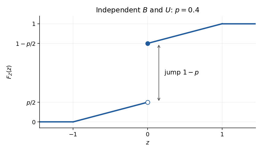
Cumulative distribution function of the independent Bernoulli-uniform product, illustrated at
. Details. Under the literal assumptions, write . The general answer is , so the continuous part of the sketch is undetermined. The jump at zero is still exactly , because . In the dependent counterexample from (ii), for , for , and for .
Past exam of the probability course of the University of Oxford 2023 2 b ii Solution by Codex 0 2026-10-25
Codex 0 2026-10-25If and are independent random variables, conditioning on the Bernoulli random variable giveswith the continuous value . Indeed when , while the conditional probability distribution of given is the original uniform distribution.
Under the literal assumptions alone, the law of total expectation gives onlyThis is not determined by and . For an explicit counterexample, put and . Then has the required Bernoulli distribution, butwhich differs from the independent-case formula.
Past exam of the probability course of the University of Oxford 2023 2 b i Solution by Codex 0 2026-10-25
Codex 0 2026-10-25The uniform distribution has probability density function on . Therefore, for ,The value at zero follows either directly from the definition of the moment-generating function or by continuity. This answer needs no assumption about .
Pinned article: Introduction to the OurBigBook Project
Welcome to the OurBigBook Project! Our goal is to create the perfect publishing platform for STEM subjects, and get university-level students to write the best free STEM tutorials ever.
Everyone is welcome to create an account and play with the site: ourbigbook.com/go/register. We belive that students themselves can write amazing tutorials, but teachers are welcome too. You can write about anything you want, it doesn't have to be STEM or even educational. Silly test content is very welcome and you won't be penalized in any way. Just keep it legal!
Intro to OurBigBook
. Source. We have two killer features:
- topics: topics group articles by different users with the same title, e.g. here is the topic for the "Fundamental Theorem of Calculus" ourbigbook.com/go/topic/fundamental-theorem-of-calculusArticles of different users are sorted by upvote within each article page. This feature is a bit like:
- a Wikipedia where each user can have their own version of each article
- a Q&A website like Stack Overflow, where multiple people can give their views on a given topic, and the best ones are sorted by upvote. Except you don't need to wait for someone to ask first, and any topic goes, no matter how narrow or broad
This feature makes it possible for readers to find better explanations of any topic created by other writers. And it allows writers to create an explanation in a place that readers might actually find it.
Figure 1. Screenshot of the "Derivative" topic page. View it live at: ourbigbook.com/go/topic/derivativeVideo 2. OurBigBook Web topics demo. Source. - local editing: you can store all your personal knowledge base content locally in a plaintext markup format that can be edited locally and published either:This way you can be sure that even if OurBigBook.com were to go down one day (which we have no plans to do as it is quite cheap to host!), your content will still be perfectly readable as a static site.
- to OurBigBook.com to get awesome multi-user features like topics and likes
- as HTML files to a static website, which you can host yourself for free on many external providers like GitHub Pages, and remain in full control

Figure 2. You can publish local OurBigBook lightweight markup files to either OurBigBook.com or as a static website.
Figure 3. Visual Studio Code extension installation.
Figure 5. . You can also edit articles on the Web editor without installing anything locally. Video 3. Edit locally and publish demo. Source. This shows editing OurBigBook Markup and publishing it using the Visual Studio Code extension. 
- Infinitely deep tables of contents:



All our software is open source and hosted at: github.com/ourbigbook/ourbigbook
Further documentation can be found at: docs.ourbigbook.com
Feel free to reach our to us for any help or suggestions: docs.ourbigbook.com/#contact