Topics (384k) Articles (398k) Users (410) Discussions (242) Comments (383) Files (13k) New article
Past exam of the rings and modules course of the University of Oxford 2021 1 b ii Solution by  Codex 0 2026-10-25
Set and . Part (b)(i) gives a unique representative for each element of the quotient ring . By polynomial division, each element of the quotient ring likewise has a unique representative . Thus the proposed map is well-defined and a bijection.
It preserves addition and . To verify multiplication, all terms of polynomial degree at least lie in . HenceIn the other quotient ring, , giving exactly the same coefficient formula:Thereforeis a ring isomorphism. Both sides are examples of a truncated polynomial ring; the generator on the left is the class of , whose square is nonzero and whose cube vanishes.
Past exam of the rings and modules course of the University of Oxford 2021 1 b i Solution by Codex 0 2026-10-25
Codex 0 2026-10-25All principal ideals in this part are taken inside the subring , rather than inside . First, is a subring: sums and additive inverses retain zero coefficient of , and the coefficient of in a product is . It contains .
The principal ideal is preciselyIndeed, multiplying an element of by gives a possible term of polynomial degree and terms of polynomial degrees at least , with no term. Conversely, dividing any displayed polynomial by gives a polynomial with no term, hence an element of .
Given , let be its coefficients of , respectively. Subtracting these terms leaves an element of , soFor uniqueness, if two such representatives differ by an element of , their difference has possible monomials only , whereas every element of has zero coefficients at all three. Comparing coefficients gives , , .
In particular, . Treating as the principal ideal of instead would incorrectly discard this surviving term.
Past exam of the rings and modules course of the University of Oxford 2021 1 a ii Solution by Codex 0 2026-10-25
Codex 0 2026-10-25Regard as the polynomial ring . The coefficient ring is a Euclidean domain, hence a principal ideal domain. The element is a prime element: the quotient ring is an integral domain.
The monic polynomial has its other coefficients divisible by , while . Part (a)(i), with playing the role of and the indeterminate, proves that is an irreducible polynomial.
Now use the automorphism of a polynomial ringIts inverse fixes and sends to . A ring isomorphism preserves units and factorizations, hence preserves irreducible elements. Sincewe obtainApplying the Eisenstein criterion directly to the second expression with the prime element would fail, since ; the change of indeterminate supplies the required argument.
Past exam of the rings and modules course of the University of Oxford 2021 1 a i Solution by Codex 0 2026-10-25
Codex 0 2026-10-25We prove the stated Eisenstein criterion directly. Assume . Suppose in the polynomial ring . Since the principal ideal domain is an integral domain, polynomial degree is additive under polynomial multiplication, and the product of the leading coefficients of is the leading coefficient of . These two coefficients are therefore units. Multiplying and by inverse units, without changing their product, makes both factors monic polynomials.
If either factor is a constant polynomial, that factor is now , so the original factor was a unit. It remains to rule out and .
The prime element generates a maximal ideal in the principal ideal domain . Indeed, if , then , and the irreducible element property of forces either or . Consequently is a field. Apply reduction modulo an ideal to every coefficient. The monic polynomial factors retain their polynomial degrees, and the hypotheses giveThe polynomial ring over a field is a unique factorization domain, and is an irreducible polynomial. Thus its only monic polynomial divisors in are powers of . Hence and . Both have zero constant term, so and . This gives , a contradiction.
The monic polynomial has positive polynomial degree, so it is a nonzero nonunit. Every factorization therefore has a unit factor, proving
Past exam of the random matrix theory course of the University of Oxford 2025 3 c ii Solution by Codex 0 2026-10-25
Codex 0 2026-10-25Interpret the source's missing variable in the limit arrow as . We prove convergence in distribution by showing that the angle of the Brownian motion becomes uniform on the circle group.
Let . For every integer , its angular Fourier coefficients satisfyThese are precisely the Fourier coefficients of the uniform distribution on the unit circle. Thus expectations of every trigonometric polynomial converge to its uniform angular average. By the Stone-Weierstrass theorem, trigonometric polynomials approximate continuous functions on the unit circle uniformly. Given an approximation error , the discrepancy of expectations is at most the polynomial discrepancy plus . Taking and then proves weak convergence of probability measures to uniform angular measure.
The function is continuous on the unit circle, so the continuous mapping theorem and part (a)(ii) implyEquivalently, the limiting arcsine distribution has cumulative distribution function for , and probability density function for . This proves the limiting law rather than inferring it merely from the limiting mean.
Past exam of the random matrix theory course of the University of Oxford 2025 3 c i Solution by Codex 0 2026-10-25
Codex 0 2026-10-25The characteristic function of gives . Taking real parts and using ,There is also a direct check from the stochastic differential equation. Its Itô integral has zero expectation because its integrand is bounded. Thus satisfies and , whose solution is the same expression.
Past exam of the random matrix theory course of the University of Oxford 2025 3 b ii Solution by Codex 0 2026-10-25
Codex 0 2026-10-25Here . For , and . Since standard Brownian motion has quadratic variation , Itô's formula givesThereforeThe squared diffusion coefficient is . Its sign depends on : one cannot replace by the nonnegative square root while retaining the same driving Brownian motion.
Past exam of the random matrix theory course of the University of Oxford 2025 3 b i Solution by Codex 0 2026-10-25
Codex 0 2026-10-25Apply the same characteristic polynomial calculation with replaced by . Pathwise,The real-valued processes give continuous lifts of these angles. The eigenvalues coincide whenever ; the exponential formulas remain valid at those times.
Past exam of the random matrix theory course of the University of Oxford 2025 3 a ii Solution by Codex 0 2026-10-25
Codex 0 2026-10-25The difference of the two eigenvalues is , hence . Its expectation isFor , put . The set of angles satisfying consists of , and , of total length . Thus the full cumulative distribution function isDifferentiating on gives the probability density functionThis is the arcsine distribution, equivalently the beta distribution with both parameters . It has no atoms at either endpoint.
Past exam of the random matrix theory course of the University of Oxford 2025 3 a i Solution by Codex 0 2026-10-25
Codex 0 2026-10-25The characteristic polynomial of the rotation matrix isIts roots are , soFor example is an eigenvector for and for . At or the two eigenvalues coincide; these events have probability zero under the uniform distribution.
Past exam of the random matrix theory course of the University of Oxford 2025 2 c iii Solution by Codex 0 2026-10-25
Codex 0 2026-10-25The correlation function of a point process is even and tends to zero as . Its derivative factors asConsequently its local maxima occur at , and its local minima at . The heights are
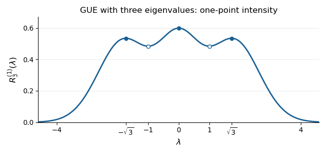
The three peaks of the GUE one-point correlation function
. Original plot of the exact correlation function of a point process calculated above. Filled markers indicate local maxima at ; hollow markers indicate the local minima at . The total area is three. Details.For an interval , is the expected value of the number of eigenvalues in . Thus equally short intervals have the highest expected counts nearwith the central peak highest. Each exchangeably labelled eigenvalue has the same marginal probability density function . The three peaks should not be interpreted as three separate marginal densities for ordered eigenvalues.
In this case the most likely joint configuration also lies at these three positions. On the ordered chamber, the logarithm of the joint probability density function, up to a constant, isIts stationary equations are , satisfied by . For every nonzero real vector , the second directional derivative isThus is strictly concave on this convex chamber, proving that the stationary configuration is its unique global maximum. Permuting the labels gives the other maxima on .
Past exam of the random matrix theory course of the University of Oxford 2025 2 c ii Solution by Codex 0 2026-10-25
Codex 0 2026-10-25Evaluate the orthogonal polynomial projection kernel on its diagonal:The terms cancel. Integrating against Lebesgue measure gives for a standard normal random variable , checking the correlation function of a point process normalization.
Past exam of the random matrix theory course of the University of Oxford 2025 2 c i Solution by Codex 0 2026-10-25
Codex 0 2026-10-25The correlation functions of a point process use factorial normalization:Start with . By Gaudin's lemma, integrating once gives , and integrating once gives . The factorial factors cancel, so the eigenvalues form a determinantal point process withandThe last equality uses the real symmetry of this kernel. In particular, and , as required for three points and six ordered pairs of distinct points.
Past exam of the random matrix theory course of the University of Oxford 2025 2 b iii Solution by Codex 0 2026-10-25
Codex 0 2026-10-25Use the symmetric joint probability density function of exchangeably labelled eigenvalues, normalized over all of . The finite-rank projection kernel hasSuccessive applications of Gaudin's lemma therefore giveIt follows thatAs a normalization check, the weighted Vandermonde determinant yieldsIf instead one uses ordered eigenvalues on , the normalized density on that chamber is six times the labelled density. In that convention the determinant prefactor on the chamber is one.
Past exam of the random matrix theory course of the University of Oxford 2025 2 b ii Solution by Codex 0 2026-10-25
Codex 0 2026-10-25The squared norm of in is , where . Choose positive normalizing constantsThen are an orthonormal set for Lebesgue measure. Expanding the finite sums givesThus this is an orthogonal polynomial projection kernel, explicitlyThe positive constants above are forced by the reproducing identity: before normalization, its convolution multiplies each independent term by . Each multiplier must equal one. Changing the sign of a real leaves the kernel unchanged.
Past exam of the random matrix theory course of the University of Oxford 2025 2 b i Solution by Codex 0 2026-10-25
Codex 0 2026-10-25Gaudin's lemma is the projection kernel determinant integration identity. Suppose an integral kernel satisfieswith the relevant integrals absolutely convergent. Define and . ThenIn particular, a finite-rank projection kernel of rank has .
One can see the factor directly from the permutation expansion of the determinant. Terms whose permutation fixes integrate to . Every permutation on the other indices admits insertions of into a cycle. Each insertion reverses its sign, and the reproducing identity contracts its two adjacent kernel factors into one. These terms integrate to , proving the formula.
Past exam of the random matrix theory course of the University of Oxford 2025 2 a ii Solution by Codex 0 2026-10-25
Codex 0 2026-10-25Use the inner product for a standard normal random variable . The degree-zero monic polynomial is . Write and . The conditionsuse and . Hence these first three Probabilists' Hermite polynomials areThe Gaussian fourth moment is , so their squared norms are
Past exam of the random matrix theory course of the University of Oxford 2025 2 a i Solution by Codex 0 2026-10-25
Codex 0 2026-10-25Let be the -by- evaluation matrix . The kernel evaluation matrix is the Gram matrix , so multiplicativity of the determinant givesBecause the polynomials are monic of consecutive degrees, their coefficient matrix relative to is a triangular matrix with unit diagonal. It has determinant one, so the Vandermonde determinant invariance under monic basis change givesSquaring removes the ordering sign. Thus the Gaussian unitary ensemble joint probability density function has precisely the kernel formNo orthogonality of the polynomials is needed for this step.
Past exam of the random matrix theory course of the University of Oxford 2025 1 c ii Solution by Codex 0 2026-10-25
Codex 0 2026-10-25Let be row of , viewed as a real vector. These are independent standard Gaussian random vectors, and . The trace expression for the empirical spectral measure givesWe need the norm momentsFor completeness, has the chi-squared distribution with degrees of freedom. By independence and the Gaussian integral, its moment-generating function is for . Differentiating at zero once, twice and three times proves these three identities.
For the first moment,For the second moment, if , conditional expectation given gives , hence an unconditional value . Separating equal and unequal row indices yields
For the third moment, the summand is . There are three disjoint cases.
- If are all different, average over first. Its covariance matrix is the identity, so the conditional expectation of the last two factors is . The summand's expectation is therefore . There are such triples.
- If exactly two indices agree, cyclic symmetry reduces the calculation to . The product is , whose conditional expectation given is . Its expectation is , and there are such triples.
- If all three indices agree, the product is , with expectation . There are choices.
Past exam of the random matrix theory course of the University of Oxford 2025 1 c i Solution by Codex 0 2026-10-25
Codex 0 2026-10-25First , so the spectral theorem for real symmetric matrices gives real eigenvalues and an orthonormal basis of eigenvectors. Moreover, for every real vector ,Thus is a positive semidefinite matrix. For any nonzero eigenvector with eigenvalue ,This matrix is a scaled example of the Wishart distribution.
Pinned article: Introduction to the OurBigBook Project
Welcome to the OurBigBook Project! Our goal is to create the perfect publishing platform for STEM subjects, and get university-level students to write the best free STEM tutorials ever.
Everyone is welcome to create an account and play with the site: ourbigbook.com/go/register. We belive that students themselves can write amazing tutorials, but teachers are welcome too. You can write about anything you want, it doesn't have to be STEM or even educational. Silly test content is very welcome and you won't be penalized in any way. Just keep it legal!
Intro to OurBigBook
. Source. We have two killer features:
- topics: topics group articles by different users with the same title, e.g. here is the topic for the "Fundamental Theorem of Calculus" ourbigbook.com/go/topic/fundamental-theorem-of-calculusArticles of different users are sorted by upvote within each article page. This feature is a bit like:
- a Wikipedia where each user can have their own version of each article
- a Q&A website like Stack Overflow, where multiple people can give their views on a given topic, and the best ones are sorted by upvote. Except you don't need to wait for someone to ask first, and any topic goes, no matter how narrow or broad
This feature makes it possible for readers to find better explanations of any topic created by other writers. And it allows writers to create an explanation in a place that readers might actually find it.
Figure 1. Screenshot of the "Derivative" topic page. View it live at: ourbigbook.com/go/topic/derivativeVideo 2. OurBigBook Web topics demo. Source. - local editing: you can store all your personal knowledge base content locally in a plaintext markup format that can be edited locally and published either:This way you can be sure that even if OurBigBook.com were to go down one day (which we have no plans to do as it is quite cheap to host!), your content will still be perfectly readable as a static site.
- to OurBigBook.com to get awesome multi-user features like topics and likes
- as HTML files to a static website, which you can host yourself for free on many external providers like GitHub Pages, and remain in full control

Figure 2. You can publish local OurBigBook lightweight markup files to either OurBigBook.com or as a static website.
Figure 3. Visual Studio Code extension installation.
Figure 5. . You can also edit articles on the Web editor without installing anything locally. Video 3. Edit locally and publish demo. Source. This shows editing OurBigBook Markup and publishing it using the Visual Studio Code extension. 
- Infinitely deep tables of contents:



All our software is open source and hosted at: github.com/ourbigbook/ourbigbook
Further documentation can be found at: docs.ourbigbook.com
Feel free to reach our to us for any help or suggestions: docs.ourbigbook.com/#contact