Topics (384k) Articles (398k) Users (410) Discussions (242) Comments (383) Files (13k) New article
Past exam of the year 2 of the earth sciences (geology) course of the University of Oxford 2024 Paper 3 4 a Solution by  Codex 0 2026-10-25
The geomorphology of active normal faulting records a competition between accumulated tectonic displacement and the ability of erosion, transport and deposition to modify it. A hanging wall moves down relative to a footwall, producing a fault scarp, mountain-front relief, and accommodation space for a sedimentary basin. Repeated earthquakes can build a large front even though each individual surface break is much smaller.[ref]
Normal-fault geomorphic features by United States Geological Survey. The primary mapping report's table of geomorphic features lists scarps, faceted spurs, oversteepened mountain fronts and rejuvenated valley floors as common normal-slip indicators.
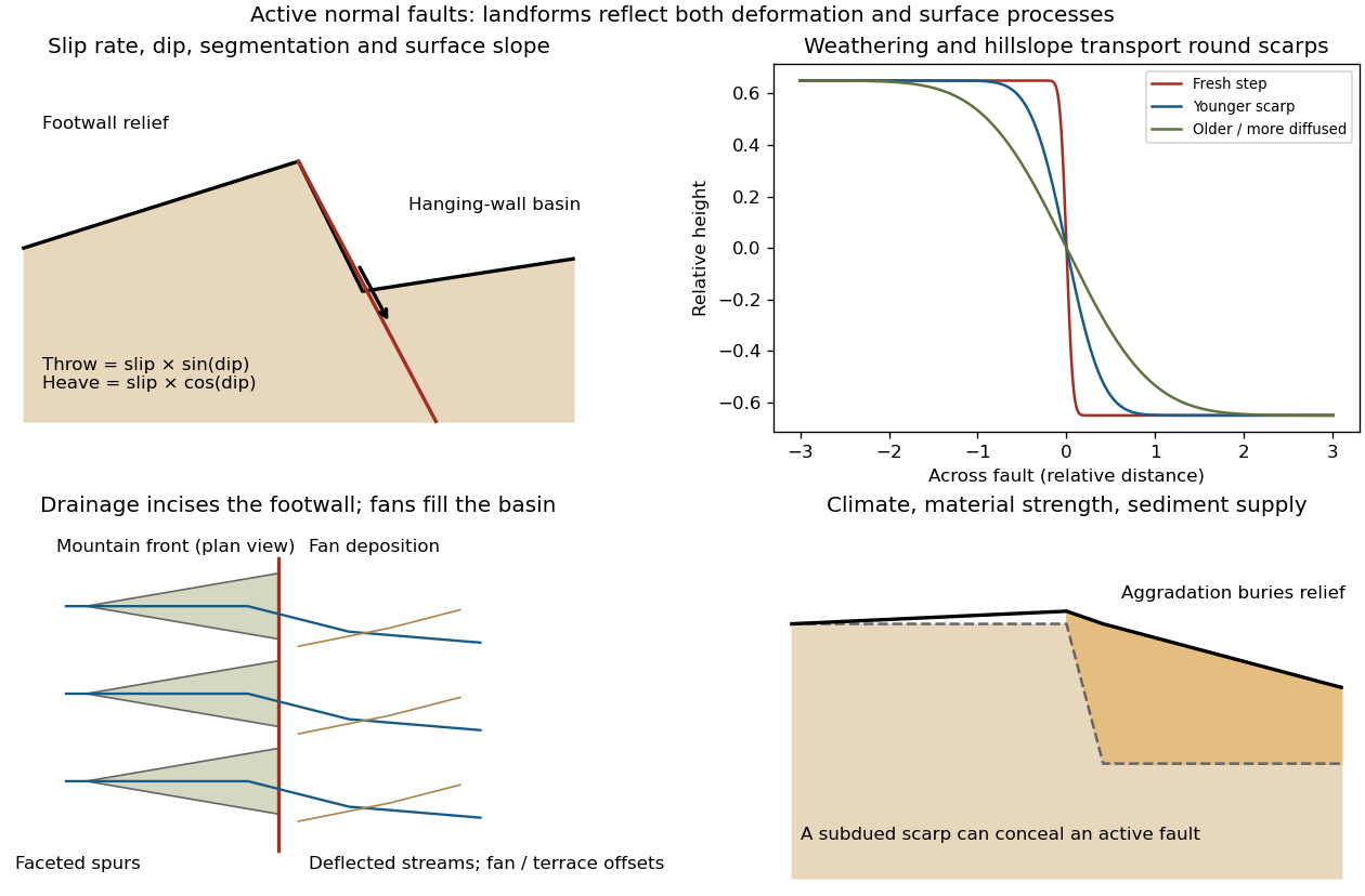
Original sketches of tectonic, erosional and depositional controls on normal-fault landforms
. The panels distinguish cumulative block displacement, progressive scarp rounding, drainage and faceted mountain fronts, and burial of a scarp by sediment. Geometries and relative scales are illustrative. Details.The principal controls and their observable effects are:
- Displacement, rate and timing. Larger single-event fault slip creates a higher fresh scarp; repeated slip builds cumulative offsets of fans and river terraces. The interval since the latest rupture controls degradation. For pure dip-slip faulting on a plane dipping , vertical fault throw is and horizontal fault heave is . Scarp height on an inclined eroded surface need not equal either the slip or the original vertical throw.
- Geometry and structural history. Fault dip, strike, curvature, segmentation, splays and along-strike variations in fault slip control scarp orientation and continuity. Linked faults can create a stepped front; synthetic and antithetic faults can create a graben. Cumulative deformation includes broad footwall uplift and hanging-wall tilting as well as a sharp break.
- Lithology and cover. Strong exposed bedrock can preserve steep scarps and fresh fault surfaces. Weak fractured rock, thick regolith and loose alluvium weather and slump more rapidly, spread deformation, and produce debris at the scarp base. Differential erosion can make a lithological front without recent tectonic movement, so a straight cliff alone is not sufficient evidence of activity.
- Climate and surface transport. Rainfall, runoff, frost action, vegetation and slope processes control scarp rounding and colluvium production. Steep new faces collapse towards stable slopes; later hillslope transport rounds the crest and fills the toe. A simple scarp diffusion model broadens a step over a length proportional to , but only if a suitable transport law and comparable material and climate apply.
- Drainage and sediment supply. Footwall uplift can incise channels and produce river terraces, knickpoints and triangular faceted spurs. Hanging-wall subsidence can pond drainage, deflect streams and promote alluvial fans and basin filling. Rapid aggradation can bury an active scarp, while stream incision can remove or exaggerate local relief.
- Preservation and initial landscape. Pre-existing slopes, relief, surface ages, glacial modification and human disturbance determine where offsets can be recognized. A fan abandoned long before the latest earthquake can accumulate more offset than a younger nearby surface. Compare like-age markers across a fault, and distinguish a mountain front's long history from a single event.
Useful observations therefore include scarp profiles, repeated offsets of dated surfaces, drainage organization, and continuity along strike. A high rugged front is not by itself evidence of a high present fault slip rate; conversely, a muted or buried scarp need not mark an inactive fault.
Past exam of the year 2 of the earth sciences (geology) course of the University of Oxford 2024 Paper 3 3 d Solution by Codex 0 2026-10-25
Codex 0 2026-10-25The result predicts initial failure in a uniform material under the assumed principal-stress orientations. The actual Figure 3 is a present-day NW–SE cross section through a thick, heterogeneous Alpine stack, extending to about 50 km depth. It contains near-horizontal basal stretches, curved ramps, tightly bent contacts, and steep structures in the internal zones around Viso and the Dora Maira complex. It does not show a single undeformed conjugate pair newly formed in horizontal uniform rock.
Several processes explain the departures:
- Mechanical layering and inherited weaknesses. Faults can follow weak bedding, old fault planes, or contacts with lower friction or cohesion than the surrounding rock. These can form shallow décollements linked by steeper ramps. Figure 2 explicitly distinguishes the near-surface red “geophysical bedrock” boundary at a few hundred metres from the much deeper crystalline basement beneath the Jurassic, Triassic and Permian cover. An age label or a seismic contrast alone does not establish a friction coefficient; clay-rich or evaporite detachments are possibilities to test, not lithologies proved by that drawing.
- Rotation after formation. Continuing tectonic shortening, folding, stacking and fault slip can rotate an initially optimal fault plane to steeper or shallower present-day fault dips. A steep older structure may be inherited from an earlier deformation episode rather than created at its present orientation.
- Curved faults and local stresses. Faults bend through a layered crust; local principal stress axes rotate near topography, ramps and interacting faults. The optimum angle is measured relative to the local , not necessarily to the regional horizontal direction everywhere.
- Changing strength and deformation mechanism. Spatial changes in pore fluid pressure, coefficient of friction, cohesion and temperature alter which surfaces reactivate. At depth, ductile deformation can replace frictional brittle failure, so the same new-fracture construction need not apply throughout the section.
Finally, a section shows apparent dip unless it is perpendicular to fault strike. For an ideal plane, , where is the angle between the section direction and fault strike. Obliquity can make a plane look shallower, but cannot on its own explain an apparent dip steeper than its true dip. Do not infer that each black curve is a currently active brittle earthquake fault.
Past exam of the year 2 of the earth sciences (geology) course of the University of Oxford 2024 Paper 3 3 c Solution by Codex 0 2026-10-25
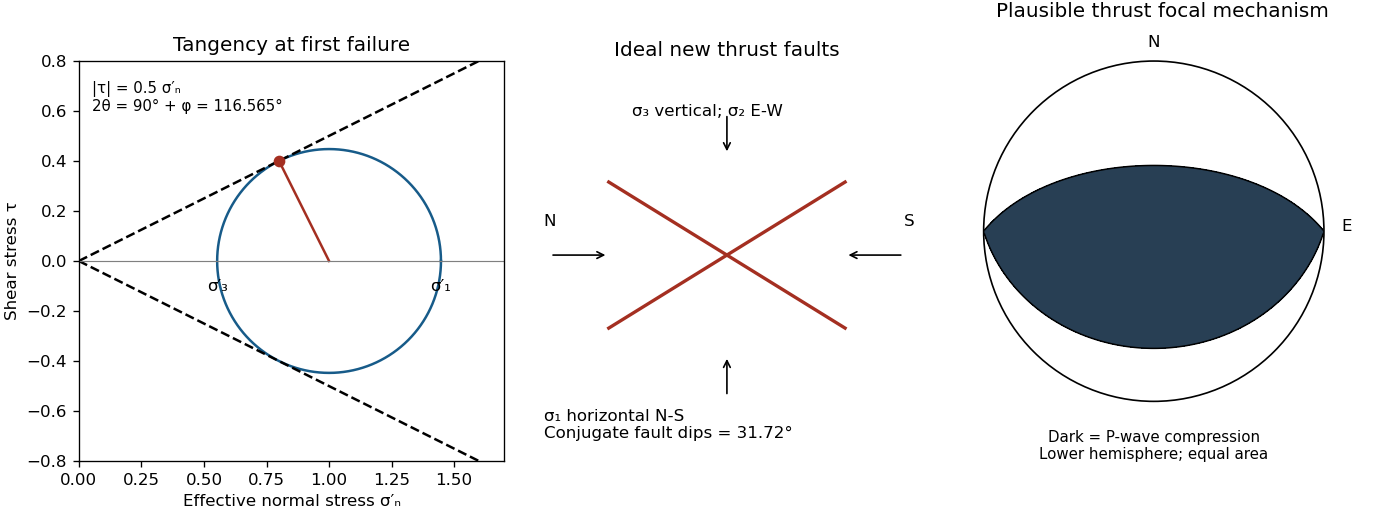
Codex 0 2026-10-25Assume an initially unfractured homogeneous isotropic material described by a linear Mohr-Coulomb failure criterion, with the given coefficient of friction representing the relevant internal friction angle. Use spatially uniform pore fluid pressure, effective stresses , and compression-positive signs. ThenThe Mohr circle in the plane has centre and radius . At first failure it is tangent to the failure envelope. The radius to the positive-shear tangent point is perpendicular to the line of slope , hence makes angle with the positive normal-stress axis.
If is the angle between the fault normal and , the stress transformation isThus , , and the angle of the fault itself to horizontal isThe two conjugate thrust faults therefore strike approximately east–west and dip about north and south. This is the fault dip, not the fault-normal angle. Both sediments and basement have the same optimum orientation under these assumptions because their stipulated friction slopes are equal; their cohesion and absolute failure stresses could still differ.
The first two panels in solution give the labeled construction. Constant cohesion shifts the straight failure envelope without changing its slope, and uniform pore fluid pressure translates the Mohr circle in normal-stress coordinates; neither changes this tangency angle. In the illustrative cohesionless case, , giving . Pre-existing weaknesses, a nonuniform stress field, anisotropic strength, or a nonlinear failure envelope invalidate the simple optimum-orientation prediction.[ref]
Stress and strength lecture notes by MIT OpenCourseWare. Lecture 10 develops the traction, pore-pressure and Mohr-circle framework; the signs and angle definitions above specify the convention used here.
Past exam of the year 2 of the earth sciences (geology) course of the University of Oxford 2024 Paper 3 3 b Solution by Codex 0 2026-10-25
Codex 0 2026-10-25A reverse or thrust fault earthquake is the expected end member: a hanging wall moves upwards relative to its footwall, accommodating north–south tectonic shortening. A plausible double-couple seismic source focal mechanism has an approximately east–west fault strike, a moderately north- or south-dipping fault plane, and up-dip fault slip. For example, right-hand-rule strike , southward fault dip about , and fault rake specify a pure thrust mechanism.
In a lower-hemisphere equal-area plot, with shaded regions denoting compressional P first motions, this focal mechanism has a shaded central region and two unshaded outer lobes. The P axis is approximately horizontal north–south and the T axis approximately vertical for a symmetric idealization; for a single plane their axes are slightly tilted. The P and T axes of a double-couple seismic source need not exactly equal the regional principal stress axes. The nodal curves represent both the fault plane and its auxiliary plane; additional evidence is needed to choose between them.[ref]
Focal mechanisms or beachballs by United States Geological Survey. Lower-hemisphere compression shading and the ambiguity between the two nodal planes.
Past exam of the year 2 of the earth sciences (geology) course of the University of Oxford 2024 Paper 3 3 a Solution by Codex 0 2026-10-25
Codex 0 2026-10-25Use compression-positive principal stresses, . For the intended thrust fault regime during approximately north–south tectonic shortening, the likely orientations areA locally horizontal traction-free surface motivates taking one principal direction as vertical, while the strong north–south compression selects the maximum horizontal principal stress. The expected fault strike is then approximately east–west.
This ordering assumes the two horizontal compressions exceed the vertical principal stress. North–south shortening by itself does not establish the magnitudes of all three: if the vertical principal stress were intermediate, strike-slip faulting would instead be possible. The answer above is the simple compressional end member used in the following parts.
Past exam of the year 2 of the earth sciences (geology) course of the University of Oxford 2024 Paper 3 2 e Solution by Codex 0 2026-10-25
Codex 0 2026-10-25Assume that the intrusion has a positive magnetic susceptibility contrast, that induced magnetization dominates its remanent magnetization, and that the local present-day geomagnetic field points roughly northward and downward, as in this northern mid-latitude setting. Writewhere is the anomalous magnetic field and the last expression assumes . A total-field magnetic anomaly measures a field projection, so it need not have the same sign everywhere above a high-susceptibility body.[ref]
The 100 km east–west extent makes an approximately two-dimensional, east–west-striking body a useful model away from its ends. On a profile drawn north on the left, south on the right, the expected normally induced response has a subsidiary negative lobe on the northern side and a stronger positive lobe over the body, displaced towards the south. The northward horizontal field component makes the anomaly asymmetric; its downward component produces the dominant positive response. The field falls back towards the regional value away from the intrusion. Broad bodies can have edge shoulders or a broad central high, so the sketch represents a qualitative shape rather than one uniquely specified curve.
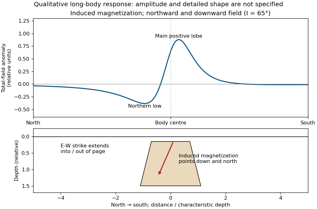
An exactly vertical inducing field would remove this north–south skew for a symmetric induced body. Real magnetic inclination and magnetic declination should be taken from a suitable geomagnetic field model for the survey date and location; no exact local value is supplied here. Strong oblique or reversed remanent magnetization can shift or reverse the lobes, and heterogeneous magnetic susceptibility, body dip and three-dimensional end effects can alter the profile. Higher magnetic susceptibility alone does not determine a unique amplitude or polarity pattern without these qualifications.
Past exam of the year 2 of the earth sciences (geology) course of the University of Oxford 2024 Paper 3 2 d Solution by Codex 0 2026-10-25
Codex 0 2026-10-25For the two negative gravity anomalies in the actual Figure 1, examine where the steepest flanks occur within the total fall into the trough. The solid upper intrusion profile has maximum slope relatively low on its flanks, close to the flat trough; its body widens downwards. The lower basin profile has maximum slope relatively high on its flanks, near the shoulders; its body narrows downwards. The dashed gradient traces and arrows mark these transitions. The signed derivative changes sign on opposite sides of a symmetric trough; a plot of gradient magnitude instead gives two positive peaks.
A shallow edge controls a relatively abrupt local change, whereas deeper geophysical density contrast spreads its effect over greater horizontal distance. Downward-narrowing geometry leaves relatively more of the anomaly associated with the shallow broad part, placing the strong flank change nearer the outer shoulders. Downward-widening geometry adds a broader deep contribution beneath the narrow outcrop, shifting the inflection towards the lower part of the trough. Thus the location of a flank's maximum slope relative to its shoulder and minimum is more useful here than the shared peak alone.
A symmetric constant-density body with vertical sides gives a symmetric negative trough with paired rounded flanks; for a broad shallow body the main slope changes occur approximately halfway down those flanks. It is intermediate between the two end members, rather than a triangular anomaly or a rectangular discontinuity. Exact fractional inflection heights depend on width, depth, burial and rounding. The following independently calculated infinite-strike models illustrate the distinction without copying Figure 1.
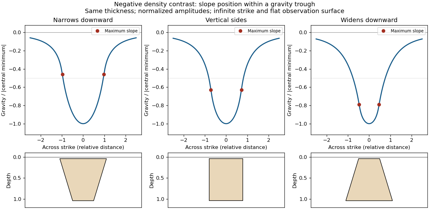
This qualitative inference assumes approximately comparable simple bodies, uniform geophysical density contrast, and a properly removed regional field. Gravity inversion is non-unique: lateral density changes, multiple bodies, and a buried top can imitate changes of wall slope. Use the seismic reflection constraints to test the interpretation.
Past exam of the year 2 of the earth sciences (geology) course of the University of Oxford 2024 Paper 3 2 c Solution by Codex 0 2026-10-25
Codex 0 2026-10-25Use the same surrounding basement density inferred in solution, carrying its unrounded value through the arithmetic. The intrusion's geophysical density contrast isThe Bouguer slab thickness needed to produce the same negative peak is thereforeThe smaller absolute geophysical density contrast requires a thicker body. This is an approximate vertical thickness and, if the top is close to the surface as drawn in Figure 1, an approximate base depth below that top. It is not an independent estimate of the intrusion's burial depth. For an infinite slab the anomaly does not depend on top depth; a buried top would require additional geometry. Finite width and the downward-widening outline in Figure 1 make 8 km a slab-equivalent estimate rather than a uniquely determined geological depth.
Past exam of the year 2 of the earth sciences (geology) course of the University of Oxford 2024 Paper 3 2 b Solution by Codex 0 2026-10-25
Codex 0 2026-10-25For a wide horizontal Bouguer slab replacing surrounding basement, use the density contrast , not the absolute sediment density:Take downward attraction as positive. The negative anomaly therefore requires . With , , and ,soThis is the requested Bouguer slab approximation: a flat observation surface, laterally infinite constant-thickness material, uniform average geophysical density contrast, and a regional anomaly already removed. The actual basin in Figure 1 narrows downwards and is finite. For a fixed maximum thickness, finite width reduces the central anomaly magnitude, so this calculation can underestimate the true magnitude of the average geophysical density contrast. It does not establish a unique basement density without the geometrical assumption.
Past exam of the year 2 of the earth sciences (geology) course of the University of Oxford 2024 Paper 3 2 a Solution by Codex 0 2026-10-25
Codex 0 2026-10-25A gravity anomaly is the difference between observed gravitational acceleration and a specified reference prediction after defined reductions. A free-air gravity anomaly, a Bouguer gravity anomaly, and a residual local gravity anomaly differ because they remove different reference contributions. State the reference ellipsoid, datum, reference density, and regional trend before interpreting an anomaly as a subsurface geophysical density contrast.
On land, tie gravimeter observations to a gravity base, calibrate them, correct instrumental drift and Earth tides, and determine station latitude and elevation accurately. Subtract latitude-dependent normal gravity . Reduce to the reference elevation using a positive free-air correction for a station above that datum: about for in metres. A simple Bouguer gravity anomaly then subtracts attraction of the intervening rock slab and adds the conventional terrain correction:with all acceleration terms expressed consistently. In SI units .
At sea, also correct vessel-motion effects, especially the Eötvös correction from east–west vessel motion and Earth rotation, and vertical ship acceleration; average or filter the moving-platform data appropriately. GPS navigation and tide information specify position and measurement height. Sea-surface measurements give a marine free-air gravity anomaly after motion, latitude, tide and height reductions. A marine Bouguer gravity anomaly additionally allows for measured bathymetry and the replacement of low-density water by reference rock; the simple water-column replacement correction is positive, , relative to the sea-surface free-air value. A consistent three-dimensional bathymetric correction is preferable near irregular coasts. Remove a justified broad regional field if the intended quantity is a residual anomaly of the local body.
Past exam of the year 2 of the earth sciences (geology) course of the University of Oxford 2024 Paper 3 10 v Solution by Codex 0 2026-10-25
Codex 0 2026-10-25 Past exam of the year 2 of the earth sciences (geology) course of the University of Oxford 2024 Paper 3 10 iv Solution by Codex 0 2026-10-25
Codex 0 2026-10-25A stability boundary in a mineral activity diagram must also be stable against the third mineral. Use the common-potential test for a three-mineral activity diagram. For the two corundum-producing directions,Negative values favour corundum. For the albite-to-nepheline conversion, , so low silica activity favours nepheline and high silica activity favours albite. These comparisons give:
All three coexist at the intersection. Pairwise mass-action equations alone do not distinguish the stable segments from their metastable extensions.
Past exam of the year 2 of the earth sciences (geology) course of the University of Oxford 2024 Paper 3 10 iii Solution by Codex 0 2026-10-25
Codex 0 2026-10-25The net reaction quotient is when the solid and water activities equal one. Therefore its equilibrium line isa vertical line through the intersection of the other two. There is no dependence on , because the net reaction contains neither hydrogen ions nor sodium ions.
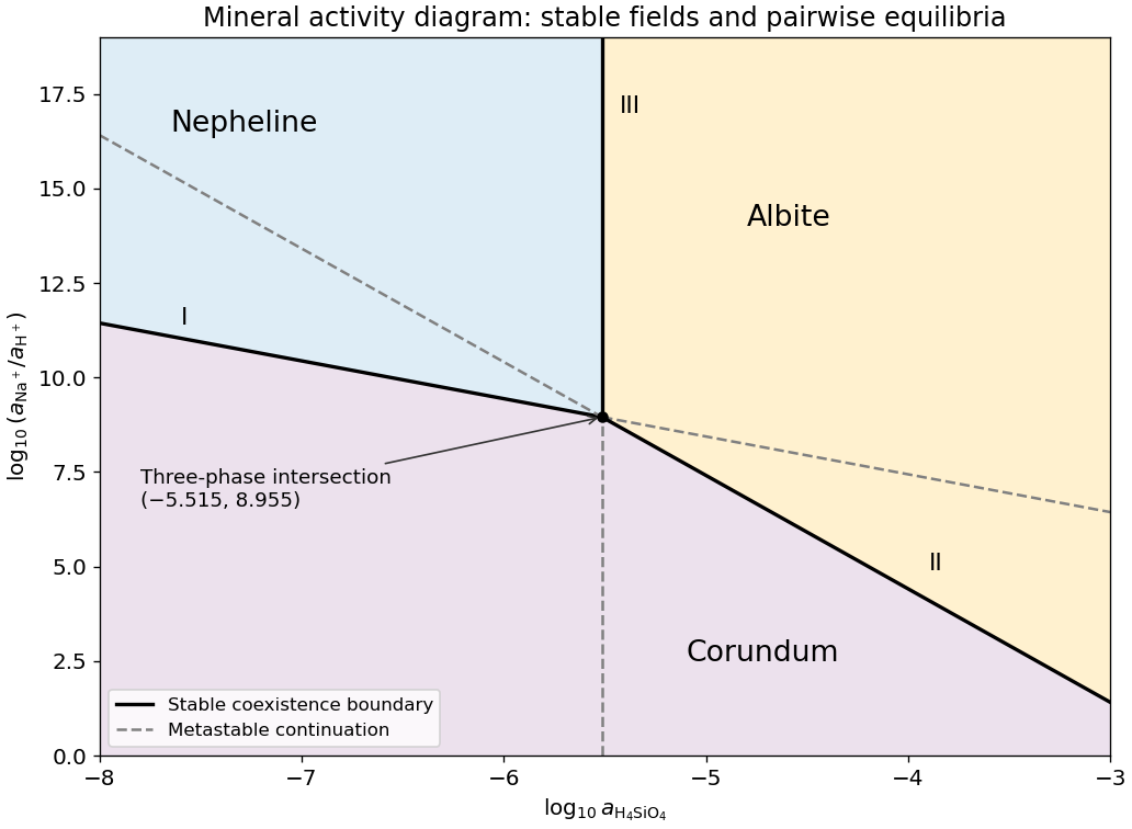
Stable and metastable mineral boundaries for the common albite-nepheline-corundum equilibrium example
. Original diagram computed from the supplied equilibrium constants. Solid lines show stable coexistence; dashed continuations are metastable. Logarithms are base ten. Details. Past exam of the year 2 of the earth sciences (geology) course of the University of Oxford 2024 Paper 3 10 ii Solution by Codex 0 2026-10-25
Codex 0 2026-10-25Subtract the nepheline–corundum reaction from the albite–corundum reaction and divide by two. In the albite-to-nepheline direction the resulting net reaction isAdditivity of the standard Gibbs energy of reaction makes the logarithms of the equilibrium constants combine with the same coefficients:This normalization is per one albite formula unit. The doubled reaction has , and reversing the reaction changes its sign.
Past exam of the year 2 of the earth sciences (geology) course of the University of Oxford 2024 Paper 3 10 i Solution by Codex 0 2026-10-25
Codex 0 2026-10-25Use base-ten logarithms and dimensionless thermodynamic activities at the stated temperature and pressure. Define and . The concentration notation is an ideal dilute-solution approximation with a consistent concentration reference.
With pure solids and unit water activity, the two reaction quotients are and . Equating them to the corresponding equilibrium constants givesThe slopes on the mineral activity diagram are and . The lines meet at , within the negative silica-logarithm range.
Pinned article: Introduction to the OurBigBook Project
Welcome to the OurBigBook Project! Our goal is to create the perfect publishing platform for STEM subjects, and get university-level students to write the best free STEM tutorials ever.
Everyone is welcome to create an account and play with the site: ourbigbook.com/go/register. We belive that students themselves can write amazing tutorials, but teachers are welcome too. You can write about anything you want, it doesn't have to be STEM or even educational. Silly test content is very welcome and you won't be penalized in any way. Just keep it legal!
Intro to OurBigBook
. Source. We have two killer features:
- topics: topics group articles by different users with the same title, e.g. here is the topic for the "Fundamental Theorem of Calculus" ourbigbook.com/go/topic/fundamental-theorem-of-calculusArticles of different users are sorted by upvote within each article page. This feature is a bit like:
- a Wikipedia where each user can have their own version of each article
- a Q&A website like Stack Overflow, where multiple people can give their views on a given topic, and the best ones are sorted by upvote. Except you don't need to wait for someone to ask first, and any topic goes, no matter how narrow or broad
This feature makes it possible for readers to find better explanations of any topic created by other writers. And it allows writers to create an explanation in a place that readers might actually find it.
Figure 1. Screenshot of the "Derivative" topic page. View it live at: ourbigbook.com/go/topic/derivativeVideo 2. OurBigBook Web topics demo. Source. - local editing: you can store all your personal knowledge base content locally in a plaintext markup format that can be edited locally and published either:This way you can be sure that even if OurBigBook.com were to go down one day (which we have no plans to do as it is quite cheap to host!), your content will still be perfectly readable as a static site.
- to OurBigBook.com to get awesome multi-user features like topics and likes
- as HTML files to a static website, which you can host yourself for free on many external providers like GitHub Pages, and remain in full control

Figure 2. You can publish local OurBigBook lightweight markup files to either OurBigBook.com or as a static website.
Figure 3. Visual Studio Code extension installation.
Figure 5. . You can also edit articles on the Web editor without installing anything locally. Video 3. Edit locally and publish demo. Source. This shows editing OurBigBook Markup and publishing it using the Visual Studio Code extension. 
- Infinitely deep tables of contents:




All our software is open source and hosted at: github.com/ourbigbook/ourbigbook
Further documentation can be found at: docs.ourbigbook.com
Feel free to reach our to us for any help or suggestions: docs.ourbigbook.com/#contact