Topics (384k) Articles (398k) Users (410) Discussions (242) Comments (383) Files (13k) New article
Past exam of the year 2 of the earth sciences (geology) course of the University of Oxford 2024 Paper 3 7 b Solution by  Codex 0 2026-10-25
Multiply the complex Fourier series by and integrate over one period. Fourier orthogonality removes every term except the one with index , givingFor general square-integrable functions, this is an orthogonal projection onto the corresponding Fourier mode. It remains valid when the expansion converges only in L2 space: integrate finite Fourier partial sums first, then pass to the limit using the Cauchy-Schwarz inequality. No unjustified pointwise exchange of an infinite series and an integral is needed.
Past exam of the year 2 of the earth sciences (geology) course of the University of Oxford 2024 Paper 3 7 a Solution by Codex 0 2026-10-25
Codex 0 2026-10-25 Past exam of the year 2 of the earth sciences (geology) course of the University of Oxford 2024 Paper 3 6 f Solution by Codex 0 2026-10-25
Codex 0 2026-10-25Choose a fixed time increment , let , and approximate by . The Backward Euler method evaluates the transport term at the new time:Rearrange to the linear systemAlthough is a singular matrix, is an invertible matrix for every . In each row, its diagonal entry is and the sum of the absolute values of its off-diagonal entries is ; hence it is a strictly diagonally dominant matrix. Its Gershgorin discs have centre and radius , excluding zero. In particular, the zero eigenvalue of becomes an eigenvalue of .
- Form once. Compute a Pivoted LU decomposition , storing the permutation matrix , the unit lower triangular matrix , and the upper triangular matrix .
- Set .
- At each step form . Solve by forward substitution, then solve by back substitution.
- Advance and repeat until the desired final time. Choose the fixed increment so the final time is an integer multiple of , or refactor if a shorter final step is used.
Both triangular solves use the factors of . The LU factorization of the singular transport matrix from part (a) is not a solver for this new linear system. No matrix inverse needs to be formed. Since and are fixed, the same LU factorization serves every step; only the right-hand side changes. A varying would give without changing these factors.
As a check, multiplying the update by givesexactly reproducing the inventory balance at the sampled times, apart from roundoff error. The Backward Euler method has temporal global error for smooth solutions, so its A-stability does not remove the need to select for accuracy.
Past exam of the year 2 of the earth sciences (geology) course of the University of Oxford 2024 Paper 3 6 e Solution by Codex 0 2026-10-25
Codex 0 2026-10-25A steady state satisfies , henceThe sign is positive on the right after rearranging the supplied equation. A solution exists exactly when lies in the column space of , which above was found to be the zero-sum vector subspace. Equivalently, multiply by the left null space vector :This condition is necessary and sufficient for an algebraic steady state, since both the column space and that zero-sum vector subspace have dimension . It expresses global conservation of mass: in the closed box model, total tracer production must balance total tracer removal. With the paper's convention , a positive is a sink and a negative is a source. If the sum is nonzero, and the inventory changes linearly in time, preventing a steady state.
When the condition holds, all algebraic steady states form the affine solution space of a linear equation , for any particular solution . The initial inventory selects one member through . For a physically admissible solution, its four concentrations must additionally be nonnegative; the compatibility condition alone imposes no such inequalities.
Past exam of the year 2 of the earth sciences (geology) course of the University of Oxford 2024 Paper 3 6 d Solution by Codex 0 2026-10-25
Codex 0 2026-10-25The null space consists of concentration patterns on which transport produces no change. Here it is the familyEvery box has the same concentration. Ocean circulation may continue, but inflow and outflow of the chemical tracer balance in each box. With these are exactly the steady states; physically admissible members have . With nonzero , adding to any particular steady state leaves its transport balance unchanged, but a null space vector alone need not balance the sources and sinks.
To identify the tracer inventory, apply conserved inventory from a left null vector. Directly summing each column givesConsequently, for the supplied ordinary differential equations,For , is a conserved quantity. The connected box model equalizes concentrations, approaching the unique member of the null space with the initial inventory:The arithmetic mean is appropriate here because the supplied matrix has zero column sums. In a general box model the conserved quantity is , where is a positive left null space vector; for physical concentrations expressed per unit volume, these weights represent the box volumes up to a common factor. One must establish the weights from the equations, rather than infer equal volumes from a schematic drawing.
Nonnegative initial concentrations remain nonnegative under transport alone. Indeed is a nonnegative matrix, sohas nonnegative entries for : it is a positive matrix semigroup. Its column sums are one by . To see why equalization occurs, set for ; then andThe right side vanishes only for constant , which in the zero-sum vector subspace means . Its strict negative bound on the unit sphere in that vector subspace gives decay to zero. Thus the matrix exponential redistributes inventory without creating negative concentrations; arbitrary prescribed sinks can still exhaust the tracer if they are allowed to act indefinitely.
Past exam of the year 2 of the earth sciences (geology) course of the University of Oxford 2024 Paper 3 6 c Solution by Codex 0 2026-10-25
Codex 0 2026-10-25Regard as a linear map . By the rank-nullity theorem and matrix rank ,All three are vector subspaces of , with the row space identified with four-component row vectors in the usual way. The null space lies in the input vector space of concentrations; the column space lies in the output vector space of concentration-change rates. Both have four coordinates, although they play different physical roles.
In this particular matrix, the row sums and column sums both vanish. Put . Then and , and the two three-dimensional vector subspaces coincide:This equality follows here from both sum identities and the dimensions of a vector space; it does not make a symmetric matrix and is not true for every square matrix.
Past exam of the year 2 of the earth sciences (geology) course of the University of Oxford 2024 Paper 3 6 b Solution by Codex 0 2026-10-25
Codex 0 2026-10-25Since is an invertible matrix, is equivalent to . The last nontrivial row gives ; the second gives ; and the first gives , so . A basis of the null space is thereforeIts single basis vector has Euclidean norm , so the unit null space basis vector is .
The pivot elements of lie in columns . Take these columns from the original matrix to obtain a basis of its column space:The fourth column is minus the sum of these three columns, and the leading three-by-three matrix minor has nonzero determinant , confirming linear independence.
Elementary row operations preserve the row space. Thus the nonzero rows of give a basis of the row space of :These basis vectors need not have unit Euclidean norm or be orthogonal. Their Euclidean norms are , respectively; the three column basis vectors have Euclidean norms .
Past exam of the year 2 of the earth sciences (geology) course of the University of Oxford 2024 Paper 3 6 a Solution by Codex 0 2026-10-25
Codex 0 2026-10-25Apply Gaussian elimination to the supplied nonsymmetric matrix,The first pivot element is , with elimination multiplier . Perform , givingThe second pivot element is , with elimination multiplier . Perform , then use the third pivot element and elimination multiplier to perform . The LU factorization isHere is a unit lower triangular matrix, hence an invertible matrix, and is an upper triangular matrix. No row interchange is needed: all three pivot elements used in elimination are nonzero. The final diagonal entry is zero, with an entirely zero last row; there is no further division by it. The three nonzero rows of are linearly independent, so the matrix rank is and is a singular matrix. Direct matrix multiplication gives .
Past exam of the year 2 of the earth sciences (geology) course of the University of Oxford 2024 Paper 3 5 e Solution by Codex 0 2026-10-25
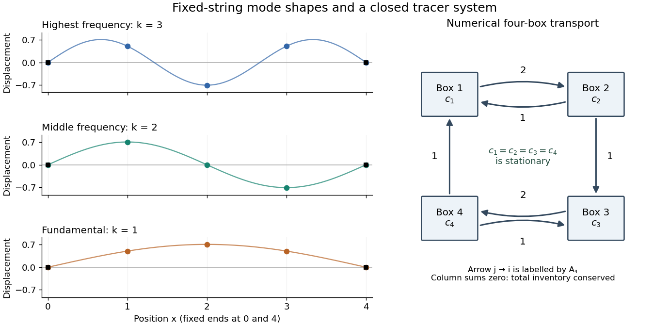
Codex 0 2026-10-25Each supplied eigenvector gives relative displacements at in a standing wave. Insert zero at to describe the whole sampled string. A real normal mode is : its shape stays fixed while its amplitude oscillates.
- is the highest-frequency resolved normal mode. Adjacent interior displacements alternate in sign: the middle point moves opposite to both outer interior points. Its interpolated shape has three lobes, corresponding to the third string normal mode.
- is the middle-frequency normal mode. The midpoint is a node of a standing wave, and the two sides move in opposite directions. It corresponds to the second string normal mode.
- is the lowest-frequency normal mode, corresponding to the fundamental frequency. All interior points move in the same direction, with greatest displacement at the centre; the only nodes of a standing wave are the endpoints in the smooth shape through these samples.
These semidiscrete fixed-string normal modes are samples of , with in the order listed. More precisely, their interior vectors are , which have unit Euclidean norm and form an orthonormal basis of . Their eigenvalues and angular frequencies obeyThus larger absolute value of a negative eigenvalue means faster oscillation, rather than faster decay. The numerical angular frequencies approximate the continuous fixed-string values ; the finite difference spatial approximation changes them. Only three independent interior normal modes exist on this grid, and any interior displacement or initial velocity vector can be expanded in this orthonormal basis.
Past exam of the year 2 of the earth sciences (geology) course of the University of Oxford 2024 Paper 3 5 d Solution by Codex 0 2026-10-25
Codex 0 2026-10-25For each row, a Gershgorin disc has centre and radius . Here and , so the Gershgorin circle theorem givesSince is a real symmetric matrix, its eigenvalues are real. Intersecting the union of these Gershgorin discs with the real axis yieldsThis bound permits zero but does not assert a zero eigenvalue. The fixed-end Dirichlet boundary conditions exclude it: for any nonzero real vector , extend by and calculateIndeed, equality would force every adjacent value to agree with the zero endpoint. Thus is a symmetric positive-definite matrix, is a negative-definite matrix, and the eigenvalues satisfy . The same argument works for any number of interior grid points, with prefactor in the sum. The fixed string has no zero-frequency rigid translation.
Past exam of the year 2 of the earth sciences (geology) course of the University of Oxford 2024 Paper 3 5 c Solution by Codex 0 2026-10-25
Codex 0 2026-10-25The interior grid is , with fixed-end displacements . HenceUse the monic characteristic polynomial convention , where is the identity matrix. Expansion of the determinant along the first row givesThe eigenvalues are the roots of a polynomial . With the alternative determinant convention , the characteristic polynomial is because the matrix has odd size; its roots of a polynomial are unchanged.
Past exam of the year 2 of the earth sciences (geology) course of the University of Oxford 2024 Paper 3 5 b Solution by Codex 0 2026-10-25
Codex 0 2026-10-25For a nonzero, time-independent vector , substitute . Taking two time derivatives givesCancel the nonzero exponential to obtain the eigenvalue problemThus an eigenvector specifies a normal mode shape and its negative eigenvalue specifies the square of its angular frequency, . Real displacements are obtained by taking the real part, or by combining the two temporal solutions as .
Past exam of the year 2 of the earth sciences (geology) course of the University of Oxford 2024 Paper 3 5 a Solution by Codex 0 2026-10-25
Codex 0 2026-10-25Put and suppose , so there are interior grid points , . Write . The fixed ends impose homogeneous Dirichlet boundary conditions,For a sufficiently smooth displacement field, the two Taylor series at fixed time givewhere all displayed derivatives on the right are evaluated at . Adding cancels the odd terms, leaving the second-order central differenceSubstitute this finite difference into the wave equation and retain continuous time. The resulting method of lines gives coupled second-order ordinary differential equations,In particular, the first and last equations are and for . With the interior displacement vector only,Equivalently, , , and all other entries vanish. This entrywise definition also covers small , including when . The matrix is a symmetric matrix and a tridiagonal matrix. The spatial approximation has error in Big O notation; time has not yet been discretized.
Past exam of the year 2 of the earth sciences (geology) course of the University of Oxford 2024 Paper 3 4 c Solution by Codex 0 2026-10-25
Codex 0 2026-10-25Excavate across the mapped fault scarp, approximately perpendicular to its strike, at a site where young sediments record and preserve deformation. On cleaned trench walls log bedding, soil horizons, shear zones, fissure fills, buried surfaces and colluvial wedges. Correlate the same marker beds across the fault before reconstructing individual displacements.
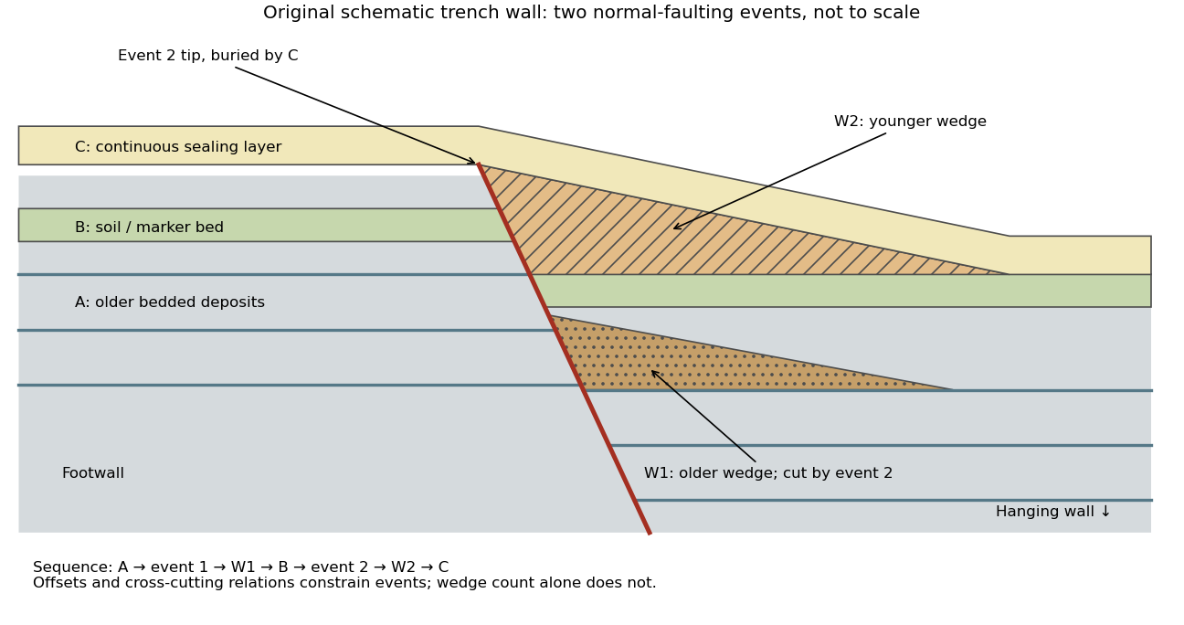
- A fault or fissure cuts older layers but terminates below an undeformed sealing deposit. The event occurred after deposition of the youngest demonstrably displaced material and before deposition of the oldest demonstrably sealing material.
- A fresh free face sheds coarse angular debris, often thickest against the scarp and thinning into the hanging wall; later finer slopewash can overlie it. A buried soil horizon between successive colluvial wedges can indicate a period of stability separating events. Fissures filled from above can preserve collapsed soil blocks or distinctive younger sediment.
- Older markers may have larger offsets than younger markers. A lower wedge or soil cut and displaced by a younger shear, then overlain by a new wedge and an intact seal, gives a cross-cutting basis for at least two events. Changes in displacement should be reconstructed across all fault strands.
- Rapid tilting, growth of accommodation space, abrupt changes in deposit thickness, and locally ponded beds can corroborate the structural evidence. Soil liquefaction structures or shaking-induced landslides may support a chronology, but do not alone prove surface rupture on the trenched fault.
In the drawing, A was faulted in event 1; W1 accumulated; B buried and stabilized that surface. Event 2 displaced A, W1 and B, after which W2 accumulated and C sealed the fault tip. Thus A records two events, B one and C none. This combination of offset and sealing relationships is stronger evidence than identifying two wedge-shaped units alone.
Bracket event ages with multiple samples just below and above the event horizons. Suitable short-lived organic material can be dated by radiocarbon dating; optically stimulated luminescence dating can constrain deposition of appropriate mineral grains. Reworked old charcoal, younger roots, incomplete bleaching, erosional gaps and time elapsed between rupture and wedge deposition must enter the age interpretation. For calendar dates, only when those deposits genuinely bracket the rupture; a radiocarbon age in years before present reverses the numerical ordering.[ref]
Introduction to paleoseismology by United States Geological Survey. “Finding Paleoearthquakes” explains disrupted layers followed by unbroken cover; “Determining the Age of a Paleoearthquake” explains dating deposits above and below the event horizon.
One earthquake can generate several debris pulses and wedges; repeated earthquakes may reuse one strand without leaving separable deposits. Erosion, bioturbation, nondeposition, lateral facies changes and upward-dying splays can hide events or mimic terminations. Confirm relationships on both trench walls and, when possible, in adjacent exposures. The result is a minimum supported event sequence with age intervals, not an assumption of perfectly periodic recurrence or one earthquake per wedge.
Past exam of the year 2 of the earth sciences (geology) course of the University of Oxford 2024 Paper 3 4 b Solution by Codex 0 2026-10-25
Codex 0 2026-10-25A surface-reaching normal fault earthquake commonly produces a down-facing step towards the hanging wall, accompanied by extension across the break. A fresh free face can expose bedrock, polish or striations, roots or offset soil. The actual rupture is usually irregular: fault slip changes along strike, separate strands overlap or step, and tension fissures, small grabens and secondary cracks distribute part of the extension.
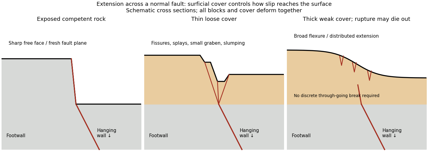
Original cross sections showing how surficial cover changes normal-fault surface rupture
. Competent exposed rock localizes a sharp free face; thin loose cover permits splays and a small graben; thick weak cover can accommodate a buried fault tip by broad flexure and distributed extension. Details.Exposed competent rock or very thin cover: a relatively narrow, sharp break can closely follow the principal fault plane. A steep free face can be recognizable immediately, then weather and shed debris. The face need not be vertical or maintain the same height along strike.
Loose granular or poorly consolidated cover: the main shear can splay upwards through alluvium or regolith. Open fissures, step-like scarps, rotated blocks, synthetic and antithetic normal faults, and a small intervening graben can form across a wider zone. Collapse and raveling quickly build colluvium at the toe. A single rupture event can therefore create several parallel breaks; counting them does not count earthquakes.
Thick weak or cohesive cover: deeper fault slip can be transferred into distributed shear strain, tilted beds, broad warping or monoclines, with tension cracks above a propagating tip. A discrete break may be attenuated or absent if the fault remains blind. Cover thickness alone is not enough to predict the response: cohesion, grain size, layering, saturation, rupture displacement and fault depth also matter. Saturated loose sediment can additionally develop soil liquefaction, sand blows or lateral spreading; these are secondary shaking effects and do not independently locate the tectonic rupture.
The observed vertical step, crack aperture and total width of disturbed ground should be measured separately. Reconstruct the total displacement across all strands and account for the original ground slope. Landslides or gravitational spreading can imitate normal-fault scarps, so map connections to the main fault and displaced markers rather than assuming every open crack is primary tectonic slip.
Pinned article: Introduction to the OurBigBook Project
Welcome to the OurBigBook Project! Our goal is to create the perfect publishing platform for STEM subjects, and get university-level students to write the best free STEM tutorials ever.
Everyone is welcome to create an account and play with the site: ourbigbook.com/go/register. We belive that students themselves can write amazing tutorials, but teachers are welcome too. You can write about anything you want, it doesn't have to be STEM or even educational. Silly test content is very welcome and you won't be penalized in any way. Just keep it legal!
Intro to OurBigBook
. Source. We have two killer features:
- topics: topics group articles by different users with the same title, e.g. here is the topic for the "Fundamental Theorem of Calculus" ourbigbook.com/go/topic/fundamental-theorem-of-calculusArticles of different users are sorted by upvote within each article page. This feature is a bit like:
- a Wikipedia where each user can have their own version of each article
- a Q&A website like Stack Overflow, where multiple people can give their views on a given topic, and the best ones are sorted by upvote. Except you don't need to wait for someone to ask first, and any topic goes, no matter how narrow or broad
This feature makes it possible for readers to find better explanations of any topic created by other writers. And it allows writers to create an explanation in a place that readers might actually find it.
Figure 1. Screenshot of the "Derivative" topic page. View it live at: ourbigbook.com/go/topic/derivativeVideo 2. OurBigBook Web topics demo. Source. - local editing: you can store all your personal knowledge base content locally in a plaintext markup format that can be edited locally and published either:This way you can be sure that even if OurBigBook.com were to go down one day (which we have no plans to do as it is quite cheap to host!), your content will still be perfectly readable as a static site.
- to OurBigBook.com to get awesome multi-user features like topics and likes
- as HTML files to a static website, which you can host yourself for free on many external providers like GitHub Pages, and remain in full control

Figure 2. You can publish local OurBigBook lightweight markup files to either OurBigBook.com or as a static website.
Figure 3. Visual Studio Code extension installation.
Figure 5. . You can also edit articles on the Web editor without installing anything locally. Video 3. Edit locally and publish demo. Source. This shows editing OurBigBook Markup and publishing it using the Visual Studio Code extension. 
- Infinitely deep tables of contents:




All our software is open source and hosted at: github.com/ourbigbook/ourbigbook
Further documentation can be found at: docs.ourbigbook.com
Feel free to reach our to us for any help or suggestions: docs.ourbigbook.com/#contact