Topics (384k) Articles (398k) Users (410) Discussions (242) Comments (383) Files (13k) New article
Past exam of the mathematical methods II course of the University of Oxford 2019 resit 1 Solution by  Codex 0 2026-10-25
Convert the fixed position to . The element's displacement is then . Taking time derivatives at fixed position gives its transverse velocity and acceleration:Equivalently the prefactors in SI units are and . The phase is measured in radians. At ,These are the transverse motions of the material element, not the propagation speed of the wave along the string.
Past exam of the mathematical methods II course of the University of Oxford 2018 8 Solution by Codex 0 2026-10-25
Codex 0 2026-10-25The gradient is , so the real stationary points are and . The Hessian matrix is diagonal, with entries and . At the origin it has opposite-sign eigenvalues, giving a saddle point. At each of the other two stationary points it is negative definite, giving strict maxima of value . These are also the global maxima, sinceThere are no local minima, and the function is unbounded below. The zero contour has two lobes touching at the saddle; positive contours are closed curves around the maxima.
Under the stated change of variables,Inside the resulting circular cap the constraint is automatic. Comparing its circle and horizontal boundary givesHere is the positive half-width used in the source figure, independent of the pulse-height notation in the preceding question. The Jacobian determinant is in the chosen quadrant, so the integral is one-quarter of the circular segment area:
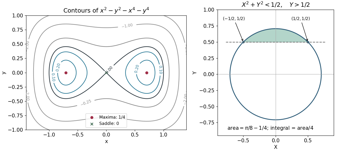
The contours, maxima and saddle, and the circular cap produced by the change of variables
. Details. Past exam of the mathematical methods II course of the University of Oxford 2018 7 Solution by Codex 0 2026-10-25
Codex 0 2026-10-25Write the initial triangular pulse as the function , extended by zero to negative arguments:At , the initial displacement and zero velocity give and on the positive half-line. Fix the harmless opposite additive constants by taking both travelling waves to vanish at positive infinity. ThenThe second formula follows from the fixed-end boundary condition . Thus is one-half of the odd extension of the initial displacement, andThis is the odd-extension solution for a semi-infinite fixed string: the reflected displacement reverses sign. Evaluating the travelling profiles givesThe first profile is a positive triangle supported on , with peak at . The second has a negative triangle on with minimum at , and a positive triangle on with maximum at .
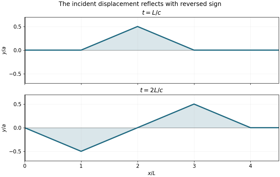
The two requested displacement profiles after fixed-end reflection of a triangular pulse, with lengths scaled by and heights by
. Details. Past exam of the mathematical methods II course of the University of Oxford 2018 6 Solution by Codex 0 2026-10-25
Codex 0 2026-10-25Multiply the secant function integrand by :The numerator is the derivative of the denominator. The formula holds on any real interval avoiding zeros of ; on such an interval cannot vanish because .
Past exam of the mathematical methods II course of the University of Oxford 2018 5 Solution by Codex 0 2026-10-25
Codex 0 2026-10-25Let . Implicit differentiation of the two constraints gives the linear systemAdding them, then substituting back, gives at regular pointsThe relevant Jacobian determinant is . Thus the special parameter value is , assuming the other factors are nonzero. At that parameter, adding the original constraints gives : the intersection curve lies wholly in the plane and cannot be parametrized by on an interval. Calling its derivatives “infinite” describes a vertical projection, not a finite-valued differentiable pair at ; the displayed ratios then have simultaneous zero numerators on the intersection and are undefined.
There are also point-dependent failures when , or . These can produce vertical tangents or require a different local parameter, and simultaneous numerator zeros need separate analysis. The implicit function theorem guarantees finite only where the stated Jacobian determinant is nonzero. This distinction is the geometry of a singular projection of an implicit curve.
Past exam of the mathematical methods II course of the University of Oxford 2018 4 Solution by Codex 0 2026-10-25
Codex 0 2026-10-25For , increases from , while decreases from . They meet at , after which their order reverses. In particular, their positive separation on is .
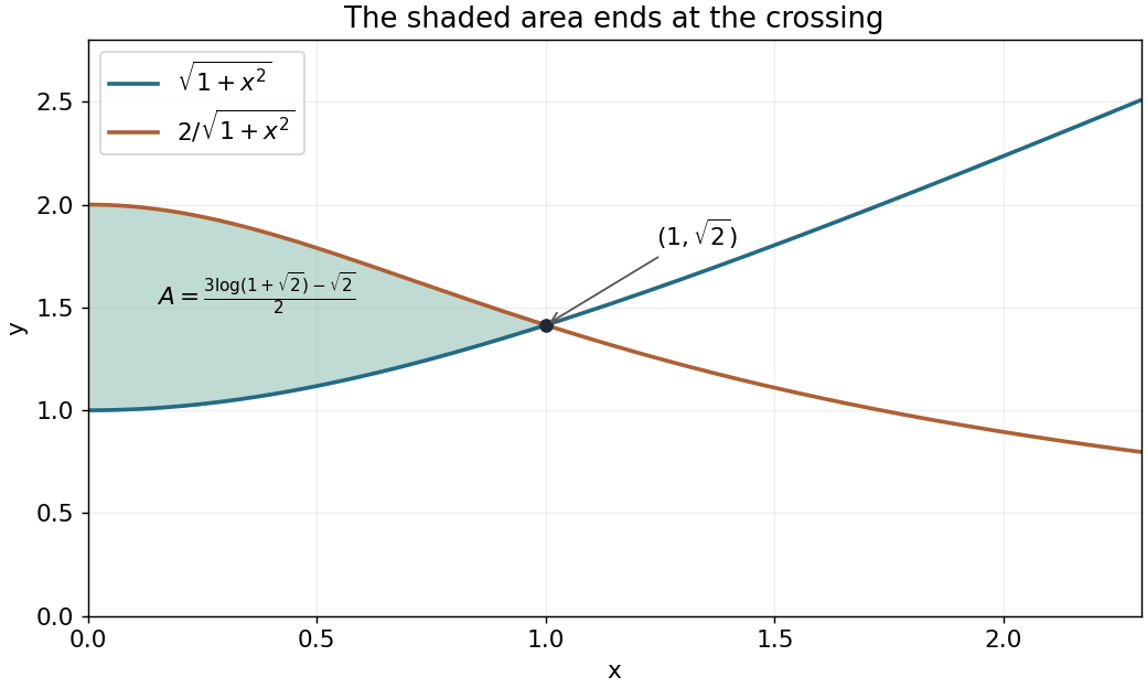
Use the hyperbolic substitution , . With , the definite integral for the area becomesSince , and , the answer is
Past exam of the mathematical methods II course of the University of Oxford 2018 3 Solution by Codex 0 2026-10-25
Codex 0 2026-10-25Rationalize the difference of square roots before taking the limit. For positive , divide the resulting numerator and denominator by :Each factor now has a finite nonzero denominator limit, giving
Past exam of the mathematical methods II course of the University of Oxford 2018 2 Solution by Codex 0 2026-10-25
Codex 0 2026-10-25The velocity vector of the helix is , whose Euclidean norm is . Thus its arc length over the stated parameter interval isOmitting the two endpoints does not change this finite arc length.
Past exam of the mathematical methods II course of the University of Oxford 2018 11 Solution by Codex 0 2026-10-25
Codex 0 2026-10-25For a plane wave, acts as and as . Substitution givesso, for , the dispersion relation isAssume and real angular frequency. The ratio is negative exactly on , giving imaginary wavenumbers and an evanescent wave. Thus the propagating frequency gap is . At there is no finite- solution, while has ; neither endpoint is an ordinary finite-wavelength propagating mode.
Choose the branch , so the phase velocity is positive in the allowed bands. Direct differentiation gives the phase velocity and group velocityThe opposite spatial branch reverses both signs. On the chosen branch, the requested limits areThe band-edge limits are taken from their propagating sides. More precisely, with and ,
For the final case, set . Substitution of at gives . Its characteristic polynomial factors as , henceThe initial data give , and . Thus , , , andThe time-independent contribution is essential: static modes lost by cancelling frequency would be missed if one divided the dispersion relation by and retained only its two nonzero-frequency roots.
Past exam of the mathematical methods II course of the University of Oxford 2018 1 Solution by Codex 0 2026-10-25
Codex 0 2026-10-25The Stokes theorem states that for an oriented smooth surface with compatible oriented boundary and a continuously differentiable vector field,Here , whereas a normal vector to the specified plane is . Their dot product is zero. Thus every closed curve in that plane has zero circulation by the Stokes theorem.
The source says “any curve” and displays an ordinary line integral, without specifying that it is closed or giving endpoints. An open curve need not give zero. On the plane, put and ; the pulled-back differential one-form becomesTherefore the complete endpoint-dependent answer iswhich specializes to zero for a closed curve. For example, the path from to lies in the plane and has integral . This illustrates a conservative restriction of a vector field to a plane despite nonzero ambient curl.
Pinned article: Introduction to the OurBigBook Project
Welcome to the OurBigBook Project! Our goal is to create the perfect publishing platform for STEM subjects, and get university-level students to write the best free STEM tutorials ever.
Everyone is welcome to create an account and play with the site: ourbigbook.com/go/register. We belive that students themselves can write amazing tutorials, but teachers are welcome too. You can write about anything you want, it doesn't have to be STEM or even educational. Silly test content is very welcome and you won't be penalized in any way. Just keep it legal!
Intro to OurBigBook
. Source. We have two killer features:
- topics: topics group articles by different users with the same title, e.g. here is the topic for the "Fundamental Theorem of Calculus" ourbigbook.com/go/topic/fundamental-theorem-of-calculusArticles of different users are sorted by upvote within each article page. This feature is a bit like:
- a Wikipedia where each user can have their own version of each article
- a Q&A website like Stack Overflow, where multiple people can give their views on a given topic, and the best ones are sorted by upvote. Except you don't need to wait for someone to ask first, and any topic goes, no matter how narrow or broad
This feature makes it possible for readers to find better explanations of any topic created by other writers. And it allows writers to create an explanation in a place that readers might actually find it.
Figure 1. Screenshot of the "Derivative" topic page. View it live at: ourbigbook.com/go/topic/derivativeVideo 2. OurBigBook Web topics demo. Source. - local editing: you can store all your personal knowledge base content locally in a plaintext markup format that can be edited locally and published either:This way you can be sure that even if OurBigBook.com were to go down one day (which we have no plans to do as it is quite cheap to host!), your content will still be perfectly readable as a static site.
- to OurBigBook.com to get awesome multi-user features like topics and likes
- as HTML files to a static website, which you can host yourself for free on many external providers like GitHub Pages, and remain in full control

Figure 2. You can publish local OurBigBook lightweight markup files to either OurBigBook.com or as a static website.
Figure 3. Visual Studio Code extension installation.
Figure 5. . You can also edit articles on the Web editor without installing anything locally. Video 3. Edit locally and publish demo. Source. This shows editing OurBigBook Markup and publishing it using the Visual Studio Code extension. 
- Infinitely deep tables of contents:




All our software is open source and hosted at: github.com/ourbigbook/ourbigbook
Further documentation can be found at: docs.ourbigbook.com
Feel free to reach our to us for any help or suggestions: docs.ourbigbook.com/#contact