Topics (384k) Articles (398k) Users (410) Discussions (242) Comments (383) Files (13k) New article
Past exam of the chemistry course of the year 3 of the natural sciences course of the University of Cambridge 2022 Paper 2A Section B 24 b ii Solution by  Codex 0 2026-10-20
For weak anchoring, , use the normalized free-molecule eigenvectors and . The perturbation isIts diagonal matrix elements in this basis are both . First-order time-independent perturbation theory for the eigenvalues therefore givesHence and . The zero free translation requires taking a square root of its new eigenvalue, rather than Taylor-expanding the frequency about zero. It is not a degenerate eigenvalue in the stipulated one-dimensional two-coordinate model.
As a check, the exact squared frequencies areExpansion gives the same first-order results; the next lower-mode correction is . The perturbed eigenvectors contain small translation/stretch admixtures of order , consistent with the failure of uniform translation to remain an exact mode in orientation (1).
Past exam of the chemistry course of the year 3 of the natural sciences course of the University of Cambridge 2022 Paper 2A Section B 24 b i Solution by Codex 0 2026-10-20
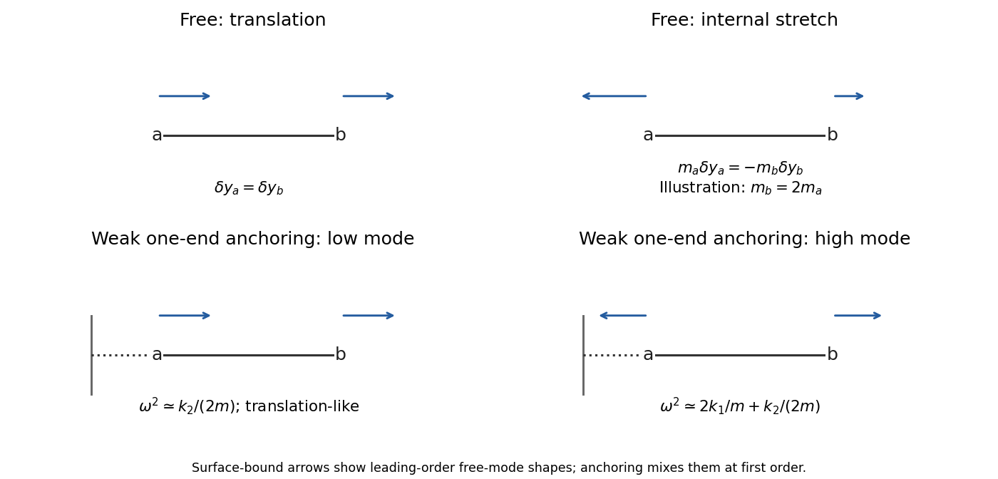
Codex 0 2026-10-20With equal masses m, the two mass-weighted Hessians areFor a uniform displacement vector ,Therefore uniform translation is not a normal mode in orientation (1) when : anchoring only one atom mixes translation with internal stretching. It is an exact normal mode displacement in orientation (2) because both atoms have identical restoring terms. Its frequency is nevertheless nonzero, ; the antisymmetric stretch has . The rigid surface breaks free translational invariance in both orientations. A vector resembling a uniform translation need not be a zero-frequency mode when the molecule is anchored.
Past exam of the chemistry course of the year 3 of the natural sciences course of the University of Cambridge 2022 Paper 2A Section B 24 a iii Solution by Codex 0 2026-10-20
Codex 0 2026-10-20Taking the Hessian of the potential with respect to mass-weighted displacements givesThe equations of motion are , so eigenvalues are squared angular frequencies. Normalized eigenvectors and frequencies areBoth vectors are in the q basis, and . The translation corresponds to equal physical displacements . The stretch has and opposite physical displacements with magnitude ratio . Ordinary frequencies are ; spectroscopic wavenumbers are .
Past exam of the chemistry course of the year 3 of the natural sciences course of the University of Cambridge 2022 Paper 2A Section B 24 a ii Solution by Codex 0 2026-10-20
Codex 0 2026-10-20Substituting givesThe shifted equilibrium coordinates satisfy . Expanding about them replaces q by displacements without changing the kinetic metric or the Hessian.
Past exam of the chemistry course of the year 3 of the natural sciences course of the University of Cambridge 2022 Paper 2A Section B 24 a i Solution by Codex 0 2026-10-20
Codex 0 2026-10-20The missing kinetic contribution is . Both atoms contribute independent translational kinetic energy before the coordinates are changed.
Past exam of the chemistry course of the year 3 of the natural sciences course of the University of Cambridge 2022 Paper 2A Section B 22 b ii Solution by Codex 0 2026-10-20
Codex 0 2026-10-20Averaging the left-minus-right differences across the three rows gives lower-state spacings of about and . Their difference is , soSimilarly, averaging successive down-column differences across the three columns gives upper-state spacings of about and . HenceUsing the first row and first column alone would give approximately and , respectively. The small inconsistency between nominally identical spacings is already present in the entries; it should be treated as limited data/model precision rather than fitted by assigning different lower-state constants to different rows. Values near for the lower state and for the upper state express the supported precision.
Past exam of the chemistry course of the year 3 of the natural sciences course of the University of Cambridge 2022 Paper 2A Section B 22 b i Solution by Codex 0 2026-10-20
Codex 0 2026-10-20Let . For a fixed row, moving one column to the right therefore givesThus adjacent-column entries decrease by the lower-state vibrational spacing, independent of the upper-state row in the ideal model. If the positive difference is instead defined as left minus right, it is . Stating the subtraction direction prevents an artificial negative vibrational frequency.
Past exam of the chemistry course of the year 3 of the natural sciences course of the University of Cambridge 2022 Paper 2A Section B 22 a iii Solution by Codex 0 2026-10-20
Codex 0 2026-10-20Successive differences remove the unknown absolute origin and the unknown initial vibrational quantum number. The five spacings are , , , and . Plot them at relative mid-indices . A straight-line fit givesThe curve reaches zero spacing at . Since a quadratic Morse progression has a spacing equal to its derivative at the interval midpoint, integrating the fitted line from the first observed relative level to estimates the energy still needed to reach the continuous limit:Thus the appropriate graphical conclusion is , not a many-digit threshold. Directly fitting a quadratic to the six measured transition positions puts its vertex at about , which checks the arithmetic but not the physical extrapolation law. The slight variation of second differences shows that extrapolating a constant anharmonicity beyond the observed range is approximate. No assignment of the arbitrary index n to an absolute upper-state v is needed.
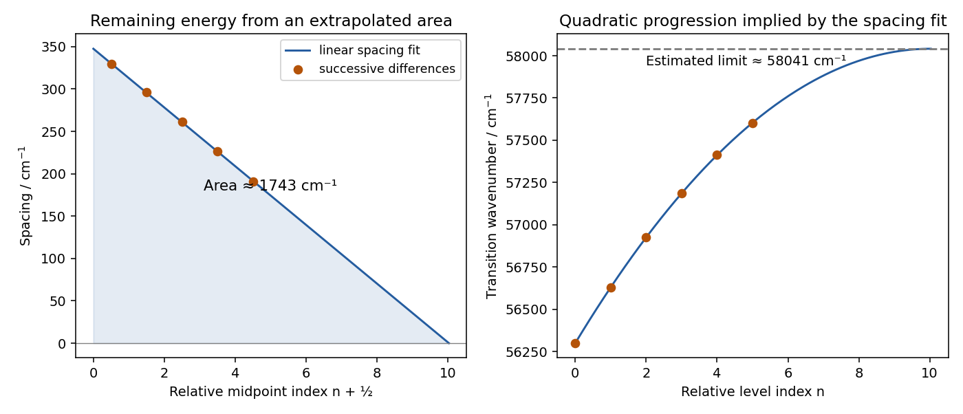
Original relative-index Birge–Sponer extrapolation and the inferred progression limit
. Details. Past exam of the chemistry course of the year 3 of the natural sciences course of the University of Cambridge 2022 Paper 2A Section B 22 a ii Solution by Codex 0 2026-10-20
Codex 0 2026-10-20Write the upper Morse oscillator term values in wavenumber units asThe spacing is . A Birge-Sponer plot therefore falls linearly in this model and can be extrapolated to zero spacing. If its horizontal coordinate is , the plotted line is . Its area from to its zero givesEquivalently a plot against has intercept and triangle area ; subtracting recovers . These conventions distinguish dissociation from the potential minimum and from the lowest vibrational level.
Measured consecutive members fix a local slope and intercept, so unobserved members can be supplied by extrapolation under an explicit spacing law. The upper-state limit on the absorption scale is . A local high-v fit can likewise estimate the remaining energy above an observed member without knowing its absolute v index. Near dissociation a real potential need not remain Morse-like, so an extrapolated triangle has model uncertainty; missing lines must not be silently assumed consecutive.
Past exam of the chemistry course of the year 3 of the natural sciences course of the University of Cambridge 2022 Paper 2A Section B 22 a i Solution by Codex 0 2026-10-20
Codex 0 2026-10-20In the Condon approximation the intensity from to contains the Franck-Condon factorThe lower ground-state vibrational wavefunction is localized near its equilibrium bond length. If the two equilibrium lengths are similar, it overlaps strongly with the upper wavefunction, but its overlap with highly excited upper vibrational states is usually small or suffers oscillatory cancellation. If the equilibrium lengths differ enough that a vertical excitation reaches the outer portion of the upper well, high- transitions can be strong while the overlap is small. Thus the two ends of a long progression are not normally both intense. This is an overlap argument, not a ban on either set of transitions; anharmonicity, a varying electronic transition moment and unusual wavefunctions can modify the intensity envelope.
Past exam of the chemistry course of the year 3 of the natural sciences course of the University of Cambridge 2022 Paper 2A Section B 21 b ii Solution by Codex 0 2026-10-20
Codex 0 2026-10-20The subbranch spacing gives , hence . Rotation about the C–I symmetry axis has momentC and I lie on this axis, so only the three hydrogens contribute to . If is the I–C–H angle, their perpendicular distances are . Taking integer hydrogen mass givesThe molecular arrangement selects the obtuse solution, so . The supplementary acute angle describes the opposite axial direction, not the bond angle to iodine. This is a rigid-geometry estimate based on an effective rotational constant and the stipulated bond length, rather than a precision equilibrium-structure measurement.
Past exam of the chemistry course of the year 3 of the natural sciences course of the University of Cambridge 2022 Paper 2A Section B 21 b i Solution by Codex 0 2026-10-20
Codex 0 2026-10-20A regularly repeated set of sharp features is characteristic of the unresolved Q subbranches of a perpendicular rovibrational band. The transition dipole is perpendicular to the symmetry axis, giving ; for the Q branch . Holding the rotational constants fixed between vibrational states cancels the term, leavingMany J transitions therefore coincide within each K-changing Q subbranch in this approximation. The different K subbranches are separated byThe P and R branches have and , respectively. Their extra J-dependent terms spread many transitions across a broad background at modest resolution. A parallel band, with , would not generate this repeated Q-subbranch spacing under the stated assumptions.
Past exam of the chemistry course of the year 3 of the natural sciences course of the University of Cambridge 2022 Paper 2A Section B 21 a iv Solution by Codex 0 2026-10-20
Codex 0 2026-10-20The largest applied field givesFor parallel polarization, adjacent allowed M values in a component are separated byAlready at this is for and for . Both exceed the stated resolution, and larger gives larger first-order spacings. The spectrometer should resolve suitable Stark components, provided their physical linewidths and signal-to-noise permit it. This predicts resolvable splittings rather than incorrectly comparing the maximum level shift directly with instrumental resolution.
Past exam of the chemistry course of the year 3 of the natural sciences course of the University of Cambridge 2022 Paper 2A Section B 21 a iii Solution by Codex 0 2026-10-20
Codex 0 2026-10-20A spectral component shifts by the difference between its upper- and lower-level Stark shifts. With , and , the supplied energy formula givesFor radiation polarized parallel to the static field, , soThus the assigned feature has no first-order splitting, whereas the features acquire symmetrically arranged magnetic-sublevel components with spacings proportional to . With perpendicular radiation, gives the corresponding different allowed pattern. Recording field-dependent spectra with specified polarization would test both the J values and the K sequence; using an individual level's shift alone would not predict the observed line positions. Higher-order shifts of the nominally unsplit feature are outside this first-order test.
Past exam of the chemistry course of the year 3 of the natural sciences course of the University of Cambridge 2022 Paper 2A Section B 21 a ii Solution by Codex 0 2026-10-20
Codex 0 2026-10-20The lines give two equations independent of :Solving yields and . The small distortion is obtained by subtracting close numbers, so its precision is considerably worse than that of .
For components in a fixed group,For example the displacement gives , while gives . Both give ; the smaller gaps are consistent after rounding. The pure rotational transitions have , so the and terms cancel. Neither nor can be determined from these zero-field lines.
Past exam of the chemistry course of the year 3 of the natural sciences course of the University of Cambridge 2022 Paper 2A Section B 21 a i Solution by Codex 0 2026-10-20
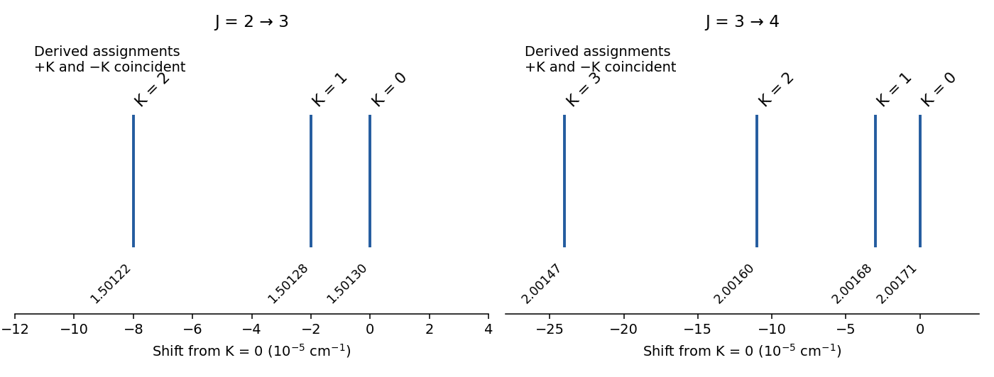
Codex 0 2026-10-20The coarse spacing is about , so . The two groups near 1.5 and therefore have and , respectively. For positive , increasing moves a component to lower wavenumber. The assignments areWithin one group, successive separations scale as . The observed gaps follow that pattern to their printed precision. There are distinct components because in the lower state; the and members remain coincident without an applied field. A high-resolution feature here is therefore not simply assigned to an arbitrary magnetic sublevel.
Past exam of the chemistry course of the year 3 of the natural sciences course of the University of Cambridge 2022 Paper 2A Section A 19 a iii Solution by Codex 0 2026-10-20
Codex 0 2026-10-20molecular mechanics evaluates a parametrized potential of atomic positions, with terms such as bond stretching, angle bending, torsion and nonbonded interactions. electrons are represented implicitly through the fitted force field, rather than by electronic orbitals, a density or an electronic wavefunction. This example is different from both preceding electronic methods.
Past exam of the chemistry course of the year 3 of the natural sciences course of the University of Cambridge 2022 Paper 2A Section A 19 a ii Solution by Codex 0 2026-10-20
Codex 0 2026-10-20Kohn-Sham equations in density functional theory use an auxiliary one-electron Hamiltonian whose effective potential depends on the density. Its orbitals construct a density representing an interacting electronic system; this is distinct from explicitly diagonalizing a large many-electron determinant Hamiltonian.[ref]
Self-Consistent Equations Including Exchange and Correlation Effects by Walter Kohn and Lu Jeu Sham. 1965, pp. A1133–A1135, ground-state effective one-electron formulation
Past exam of the chemistry course of the year 3 of the natural sciences course of the University of Cambridge 2022 Paper 2A Section A 19 a i Solution by Codex 0 2026-10-20
Codex 0 2026-10-20configuration interaction with singles and doubles (CISD) uses a linear combination of the reference Slater determinant and singly and doubly excited determinants. Its many-electron trial state is therefore not restricted to one determinant; the orbitals may be held fixed while the configuration coefficients are varied.
Past exam of the chemistry course of the year 3 of the natural sciences course of the University of Cambridge 2022 Paper 2A Section A 15 c ii Solution by Codex 0 2026-10-20
Codex 0 2026-10-20Now and the ground term is . Spin-conserving transitions to the labelled doublet excited terms are possible. Reading the diagram gives approximatelyThe first two upper terms are coincident or unresolved at this diagram's resolution. These doublet transitions should dominate over the spin-forbidden transitions to sextet or quartet levels. Their intensity still depends on vibronic or other relaxation of the Laporte rule. The plotted curves justify only approximate wavenumbers, not several-digit band positions.
Pinned article: Introduction to the OurBigBook Project
Welcome to the OurBigBook Project! Our goal is to create the perfect publishing platform for STEM subjects, and get university-level students to write the best free STEM tutorials ever.
Everyone is welcome to create an account and play with the site: ourbigbook.com/go/register. We belive that students themselves can write amazing tutorials, but teachers are welcome too. You can write about anything you want, it doesn't have to be STEM or even educational. Silly test content is very welcome and you won't be penalized in any way. Just keep it legal!
Intro to OurBigBook
. Source. We have two killer features:
- topics: topics group articles by different users with the same title, e.g. here is the topic for the "Fundamental Theorem of Calculus" ourbigbook.com/go/topic/fundamental-theorem-of-calculusArticles of different users are sorted by upvote within each article page. This feature is a bit like:
- a Wikipedia where each user can have their own version of each article
- a Q&A website like Stack Overflow, where multiple people can give their views on a given topic, and the best ones are sorted by upvote. Except you don't need to wait for someone to ask first, and any topic goes, no matter how narrow or broad
This feature makes it possible for readers to find better explanations of any topic created by other writers. And it allows writers to create an explanation in a place that readers might actually find it.
Figure 1. Screenshot of the "Derivative" topic page. View it live at: ourbigbook.com/go/topic/derivativeVideo 2. OurBigBook Web topics demo. Source. - local editing: you can store all your personal knowledge base content locally in a plaintext markup format that can be edited locally and published either:This way you can be sure that even if OurBigBook.com were to go down one day (which we have no plans to do as it is quite cheap to host!), your content will still be perfectly readable as a static site.
- to OurBigBook.com to get awesome multi-user features like topics and likes
- as HTML files to a static website, which you can host yourself for free on many external providers like GitHub Pages, and remain in full control

Figure 2. You can publish local OurBigBook lightweight markup files to either OurBigBook.com or as a static website.
Figure 3. Visual Studio Code extension installation.
Figure 5. . You can also edit articles on the Web editor without installing anything locally. Video 3. Edit locally and publish demo. Source. This shows editing OurBigBook Markup and publishing it using the Visual Studio Code extension. 
- Infinitely deep tables of contents:




All our software is open source and hosted at: github.com/ourbigbook/ourbigbook
Further documentation can be found at: docs.ourbigbook.com
Feel free to reach our to us for any help or suggestions: docs.ourbigbook.com/#contact