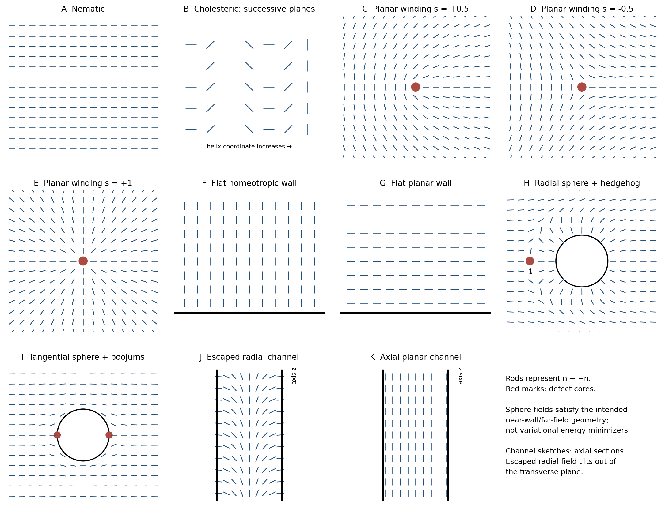
planar anchoring favors the nematic director tangent to a surface. A flat wall at $z=0$ permits uniform $\mathbf{n}=\hat{\mathbf{x}}$, as in the sketch. A rubbed surface can select one in-plane axis; degenerate planar anchoring selects only the tangent plane.

For the degenerate case, $f_s=(W/2)(\mathbf{n}\cdot \mathbf{\nu }{)}^2$ has minima at $\mathbf{n}\cdot \mathbf{\nu }=0$. A remote incompatible boundary produces elastic distortion. Tangency alone does not specify an azimuthal direction within the surface.

homeotropic anchoring favors the nematic director normal to a surface. For a flat wall at $z=0$, uniform $\mathbf{n}=\hat{\mathbf{z}}$ is a simple compatible profile, shown as perpendicular rods. If a remote wall demands another orientation, elastic bending interpolates between the boundaries.

A common surface energy is $f_s=(W/2)[1-(\mathbf{n}\cdot \mathbf{\nu }{)}^2]$, with wall normal $\mathbf{\nu }$ and $W>0$. Its minima have $\mathbf{n}$ parallel or antiparallel to $\mathbf{\nu }$. The profile is controlled jointly by this preference and Frank elastic energy.

The blue phases result when strong local chirality favors double twist that cannot fill three-dimensional space everywhere without frustration. Double-twist regions are connected through a network of nematic disclinations.

Blue phase I has body-centered cubic order and blue phase II simple-cubic order in their director/defect structures. The periodicity can cause selective optical reflection. Blue phase III is disordered or amorphous, not another ideal cubic lattice. These are structured fluid phases rather than ordinary crystals with molecules fixed to every lattice site.

A cholesteric liquid crystal is locally nematic but its nematic director rotates helically, for exampleThe sign of $q_0$ specifies handedness and $p$ is the full-turn pitch. The sketch shows rods rotating through transverse planes. This is helical orientational order, not a smectic density-layer lattice. Although an apolar director repeats physically after a half-turn, the conventional pitch denotes a full $2\pi$ turn. A pitch comparable to visible wavelengths can give selective reflection.

A liquid crystal flows while retaining partial molecular order. A nematic liquid crystal has long-range orientational order but no crystal-like positional lattice. Its local mean axis is the nematic director $\mathbf{n}$, with $\mathbf{n}\equiv -\mathbf{n}$ for an ordinary apolar nematic. Order leads to anisotropic optical and dielectric response and an elastic cost for director distortions.

Nematic order selects an axis, not a common molecular head direction or density-layer stack. The original sketch uses short rods as a coarse-grained orientation map.

Yes: carbon nanotubes can store lithium and form a porous, conducting anode network. Their external surfaces, defects and intertube spaces provide possible storage sites. Open ends and suitable defects may make internal surfaces accessible; a closed pristine tube should not be credited with its full internal area.

Axial conduction and an entangled mechanical scaffold can support either active storage or a composite electrode. Limitations include tube–tube contact resistance, low packing density, catalyst residues and large-area solid electrolyte interphase formation. Opening or functionalizing tubes may improve ion access while increasing defects and irreversible reactions. Compare reversible capacity, first-cycle efficiency, retention and full-cell lithium inventory under matched loading and voltage-window conditions. A high first-cycle capacity alone is insufficient evidence of a superior anode.

I would choose liquid-phase exfoliation of graphite into few-layer graphene, followed by controlled electrode formation. It uses bulk feedstock and preserves much of the $s{p}^2$ framework; a battery electrode does not require a wafer-sized perfect monolayer.

Disperse graphite in a compatible liquid, apply shear or sonication, and classify the dispersion to separate thin flakes from unexfoliated material. Recover and wash the selected fraction, remove contaminants and dispersants, then coat a Cu current collector with a suitably bound, porous and electrically connected film. Drying and consolidation should establish contacts without collapsing every transport pore. Characterize thickness and size distributions, residual impurities and conductivity after processing.

The advantages are solution compatibility, accessible feedstock and less basal-plane chemical disruption than oxidation–reduction routes. Limitations include a distribution of layer numbers, limited single-pass yield, flake fragmentation, solvent recovery and drying-induced restacking. Solvent toxicity and retained surfactants matter for manufacturing. In the original exfoliation study, microscopy and spectroscopy distinguished thin flakes from graphite and checked structural preservation; those controls precede any performance claim.^[ref]

Oxidation–exfoliation–reduction is another scalable route, but irreversible lattice damage and residual oxygen make conductivity and first-cycle losses separate concerns.

Separated graphene sheets offer high accessible surface area, short lithium-transport distances and a conducting network. Edges and exposed sheet faces can supply additional storage sites; mechanical flexibility can help preserve contact during cycling. These advantages can improve rate capability when electrolyte access and electronic continuity are retained.

The graphite reference composition $\mathrm{Li}{\mathrm{C}}_6$ giveswhere the host-carbon mass is used. An idealized $\mathrm{Li}{\mathrm{C}}_3$ inventory doubles this figure, but two accessible faces do not prove a reversible $\mathrm{Li}{\mathrm{C}}_3$ electrode. Binding energies, aggregation, defects and electrolyte stability determine actual storage.

Large area increases electrolyte decomposition and solid electrolyte interphase formation, consuming lithium in early cycles. Restacking reduces accessible area, low packing density reduces volumetric capacity, and residual oxygen, defects or binder can lower conductivity and active mass fraction. A broad storage-voltage profile may lower full-cell energy efficiency. Compare electrodes at matched areal loading and practical current density, reporting first-cycle efficiency, retention, voltage profile and volumetric as well as gravimetric capacity.

Clean the exposed silicon and grow a thin, high-quality SiO2 gate dielectric by controlled dry thermal oxidation. Deposit polycrystalline silicon, conventionally by low-pressure chemical vapour deposition from silane, dope it in situ or by subsequent implantation and activation, and pattern/etch it to define the two gates. Phosphorus or arsenic gives n+ polysilicon; boron gives p+ polysilicon where the selected gate-work-function process requires it. A traditional single-poly process may use a common gate doping instead; gate and source/drain doping need not be identical.

The patterned gates subsequently serve as self-alignment masks for donor-doped nMOS source/drain and acceptor-doped pMOS source/drain regions. Annealing activates these dopants. Keep the oxide thin and uniform enough for strong electrostatic control but free from pinholes and excessive leakage. A high-permittivity dielectric deposited by atomic layer deposition with a metal gate is a modern alternative, rather than the conventional polysilicon/SiO2 stack drawn.

Start with a lightly boron-doped p-type Si wafer. Define an implantation opening for the pMOS region using an oxide/nitride implantation mask, then implant donor ions, commonly phosphorus, at energies and doses giving the required well depth and concentration. An anneal activates donors and repairs damage; thermal drive-in can deepen and smooth the well profile. The donor concentration must exceed the original acceptor concentration in the well. Retain p-type material outside it for the nMOS device. Form a later n+ well contact to tie the n-well to the positive supply; the p+ substrate contact ties the substrate to ground. Diffusion from a donor source is an alternative to ion implantation and drive-in.

Measure a genuinely flat calibration reference over the same scan range, scanner position and operating conditions, then subtract its reproducible bow background from the specimen data. Retain reference flat regions outside the feature if available, fitting only those regions rather than the bulge. A scanner with independently measured vertical motion or suitable closed-loop correction reduces the instrumental uncertainty. Translating or rotating the specimen checks whether a feature follows the specimen or the scanner coordinates; independent optical or stylus profilometry can corroborate its height. For a rotationally symmetric parabola, rotation alone is not sufficient. Report drift and calibration uncertainty as part of the $200\mathrm{nm}$ height measurement.

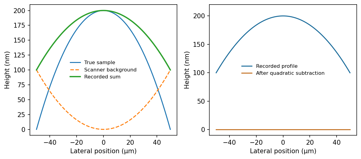
Common processing fits and subtracts a low-order polynomial background, often a quadratic surface or a polynomial for each scan line. This AFM image flattening removes scanner curvature on an assumed flat sample. Here the desired specimen signal is itself roughly quadratic, so such subtraction can remove the actual $200\mathrm{nm}$ bulge along with the artefact. The two contributions cannot be separated by polynomial fitting to this image alone. A plane subtraction removes tilt but does not independently calibrate curvature.

Scanner bow is the relevant artefact. A piezoelectric tube scanner bends to produce lateral displacement; its moving end also follows a curved vertical trajectory. Cross-coupling of lateral and vertical motion therefore gives a roughly quadratic height background even over a flat reference. Over a wide scan it can mimic or conceal a genuine parabolic sample profile; its sign depends on scanner geometry and height convention.

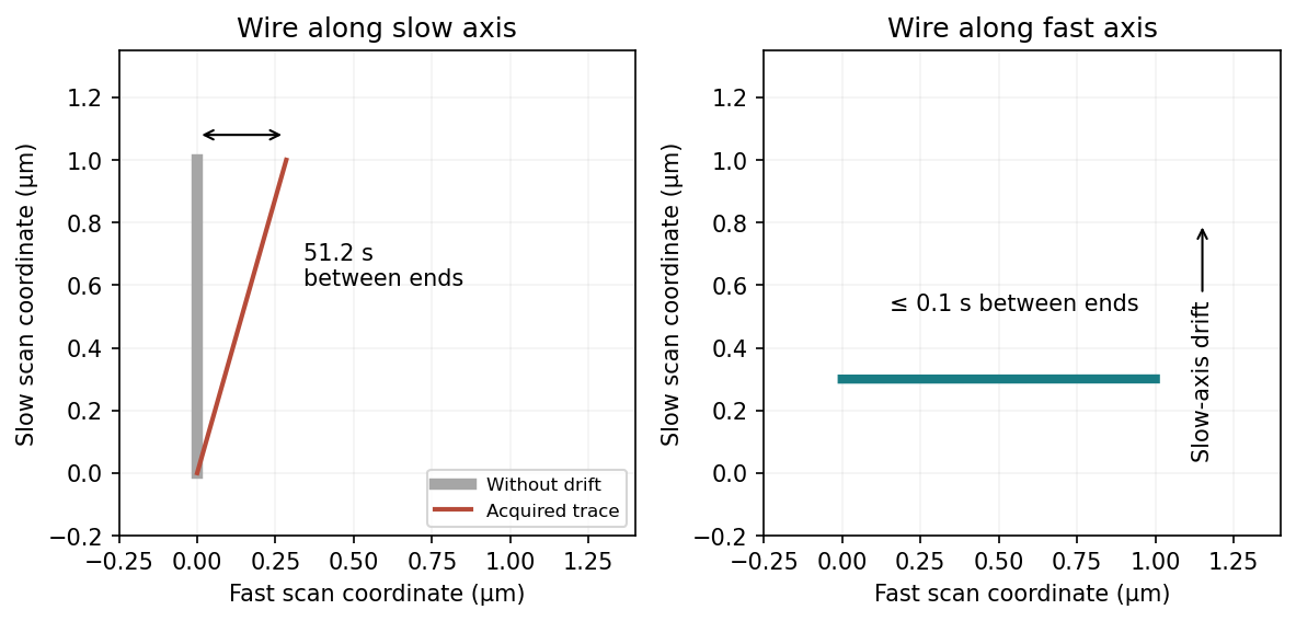
Place the wire parallel to the fast scan axis. The endpoints are then recorded in a fraction of a line period, rather than tens of seconds apart, minimizing the differential drift accumulated between them.

This does not remove drift of the wire's transverse position or apparent width between successive lines. A very thin wire parallel to the fast axis may fall between the discrete slow-axis scan lines, so a smaller scan area or denser sampling can be needed. Tip convolution, pixel resolution and feedback lag remain; trace/retrace comparisons and allowing thermal equilibration are still valuable. Increasing the scan speed indefinitely is limited by the scanner and feedback bandwidth.

One image takes $512\mathrm{s}$ if $1\mathrm{Hz}$ means one completed scan line per second. The slow-axis speed is $10/512=0.01953\mu \mathrm{m}{\mathrm{s}}^{-1}$. Recording a wire spanning $1\mu \mathrm{m}$ along that axis therefore takes $51.2\mathrm{s}$. Meanwhile the fast-axis drift is $20/3600=0.005556\mu \mathrm{m}{\mathrm{s}}^{-1}$, giving a transverse displacement of $0.2844\mu \mathrm{m}$. The apparent straight-line length isIts slow-axis projection remains $1\mu \mathrm{m}$; the overestimate refers to length along the slanted trace.

With the wire along the fast axis and drift along the slow axis, its length is acquired within one line, so $L_{\mathrm{app}}\simeq 1.000\mu \mathrm{m}$. Taking a forward sweep of $1\mathrm{s}$ across $10\mu \mathrm{m}$, the wire is crossed in $0.1\mathrm{s}$ and the perpendicular displacement is only $0.556\mathrm{nm}$. The corresponding length change is about $1.5\times 10^{-7}\mu \mathrm{m}$, far below the $19.5\mathrm{nm}$ pixel pitch. For the convention in which one hertz includes a forward and reverse sweep, that already negligible displacement halves. The slow-axis calculation still uses one completed line per second.