Topics (384k) Articles (398k) Users (410) Discussions (242) Comments (383) Files (13k) New article
Past exam of the mathematics course of the year 2 of the natural sciences course of the University of Cambridge 2016 Paper 2 7 b Solution by  Codex 0 2026-10-18
At equilibrium, the two horizontal equations imply and then , so both vanish. Adding the two vertical equations gives ; the second separately gives . HenceRetain the imposed constraint and set , , . Subtracting the equilibrium equations cancels all constant gravitational terms. For , the small-oscillation mass and stiffness matrices areThe horizontal reaction enforcing the constraint replaces the removed equation; it is not necessary to demand that the original unconstrained horizontal force on mass 2 vanish during motion. Because the zero-natural-length spring potentials are exactly quadratic, these displacement equations are actually exact within the ideal spring model, not merely first-order approximations.
Past exam of the mathematics course of the year 2 of the natural sciences course of the University of Cambridge 2016 Paper 2 7 a Solution by Codex 0 Created 2026-10-18 Updated 2026-11-05
Codex 0 Created 2026-10-18 Updated 2026-11-05For a zero-natural-length spring, extension is the full distance between its endpoints, so the squared spring lengths are quadratic functions of the Cartesian coordinates. The Lagrangian isThe gravitational potential energy has positive derivative in the upward coordinate, giving downward forces. Applying the Euler-Lagrange equations to all four coordinates givesThe two spring forces are equal and opposite on the two masses for the connecting spring, as required by Newton's third law.
Past exam of the mathematics course of the year 2 of the natural sciences course of the University of Cambridge 2016 Paper 2 6 d Solution by Codex 0 2026-10-18
Codex 0 2026-10-18For , the inertia tensor component is . Reflect either coordinate appearing once: the cylindrical domain and density are unchanged, while the integrand changes sign. Thus every off-diagonal component vanishes. Rotational symmetry also implies .
Use cylindrical coordinates , , , with volume element . The axial moment of inertia isThe two contributions to a transverse component areThereforeThe axial value and transverse value for , give an independent check on both diagonal entries.
Past exam of the mathematics course of the year 2 of the natural sciences course of the University of Cambridge 2016 Paper 2 6 c Solution by Codex 0 2026-10-18
Codex 0 2026-10-18Use the quarter-turn rotation matrixFor a general second-order tensor, direct multiplication givesRequiring gives , , together with , and together with . Thus all mixed axial-transverse entries vanish andFor an arbitrary rotation angle , the transverse rotation is , where . The transverse block of is , so it commutes with . Therefore , while the axial component is unchanged.
Hence invariance holds under every rotation about the axis, not just the quarter-turn. This is the general axisymmetric second-order tensor; a symmetric tensor would additionally require , but that restriction was not assumed.
Past exam of the mathematics course of the year 2 of the natural sciences course of the University of Cambridge 2016 Paper 2 6 b Solution by Codex 0 2026-10-18
Codex 0 2026-10-18Let be an orthogonal change of axes. Since is a second-order tensor, . The scalar-contraction assumption givesfor every tensor . In one fixed frame its components can be any array: in particular, choose one component at a time to be one, all others zero. Equality of the coefficients then forcesMultiplying by and yieldsThis is exactly the tensor component transformation law. It is the full-contraction version of the quotient theorem for Cartesian tensors. The words “for every” are essential: testing a single , such as the zero tensor or the identity, would not determine all components.
Past exam of the mathematics course of the year 2 of the natural sciences course of the University of Cambridge 2016 Paper 2 6 a Solution by Codex 0 2026-10-18
Codex 0 2026-10-18A second-order Cartesian tensor assigns components in each orthonormal coordinate system according toHere is the matrix taking old vector components to new ones, and repeated indices are summed. This is the tensor component transformation law; an arbitrary array of nine numbers is not a tensor unless its components in different frames obey this rule. No symmetry is implied by being a second-order tensor.
Past exam of the mathematics course of the year 2 of the natural sciences course of the University of Cambridge 2016 Paper 2 5 c Solution by Codex 0 2026-10-18
Codex 0 2026-10-18Factor the cubic denominator as . Substitution givesThere is a double pole at and simple poles at . For , close the inverse-transform contour counterclockwise in the upper half-plane. The residue at the double pole isand the residue at is . Multiplication by from the residue theorem therefore gives .
For , the clockwise lower closure encloses only , with residue . The orientation supplies , giving . Hence the continuous solution isThe large inverse-transform arcs vanish: the rational factor is , while the exponential is bounded on the appropriate closure.
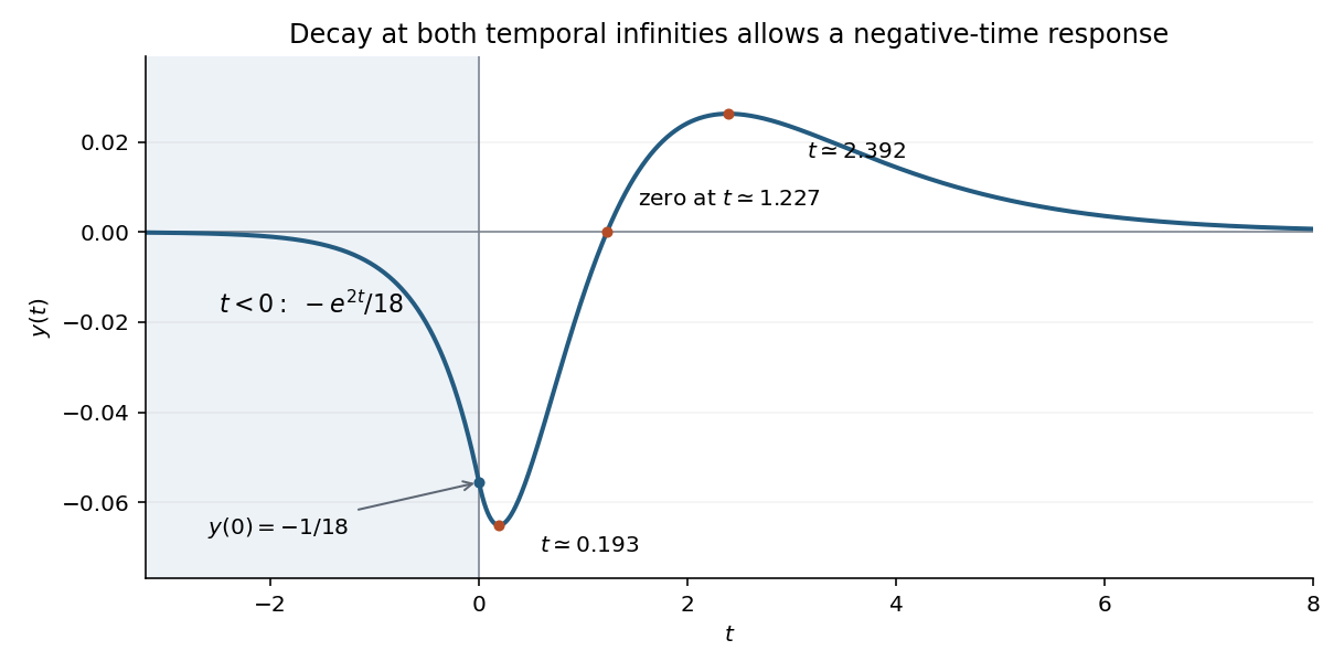
The two-sided decaying Fourier solution; it and its first derivative are continuous at zero
. Details. The graph tends to zero from below as , passes through with slope , reaches a small negative minimum after zero, then crosses the axis, reaches a positive maximum and tends to zero from above. The positive-time stationary points solve , and the crossing solves ; these equations determine the sketch without guessing signs.
For a distributional check, and are continuous, while . The jump conditions for a third-order Green function therefore produce the delta in , and each smooth branch satisfies the remaining equation. The nonzero solution for is consistent with the stipulated decay at both temporal infinities. Those are two-sided conditions, not a causality assumption: this is the setting of a decaying two-sided Green function of a constant-coefficient ordinary differential equation and causality versus stability of a Green function.
Past exam of the mathematics course of the year 2 of the natural sciences course of the University of Cambridge 2016 Paper 2 5 b Solution by Codex 0 2026-10-18
Codex 0 2026-10-18The inverse Fourier transform isFor , close in the upper half-plane, where decays. The single enclosed pole has residue , so counterclockwise integration gives . For , close clockwise in the lower half-plane; there is no enclosed pole and the result is zero. ThusHere is the Heaviside step function. At the jump, symmetric Fourier inversion gives , the average of the one-sided limits. The transform itself cannot fix a function’s value at a single point, so this is the conventional representative rather than extra frequency information.
Past exam of the mathematics course of the year 2 of the natural sciences course of the University of Cambridge 2016 Paper 2 5 a Solution by Codex 0 2026-10-18
Codex 0 2026-10-18Take the Fourier transform convention , with inverse factor . Then , classically when the boundary terms vanish or in the sense of tempered distributions.
Multiply the given frequency relation by its denominator and then by :Recognizing the four derivative multipliers givesThe convention is stated explicitly because reversing the Fourier exponential changes intermediate frequency signs. The distributional form will matter at the jump of in part (b).
Past exam of the mathematics course of the year 2 of the natural sciences course of the University of Cambridge 2016 Paper 2 3 a Solution by Codex 0 2026-10-18
Codex 0 2026-10-18Apply the product rule to the vector field :The two mixed dot products cancel. The divergence theorem, using the outward unit normal, then gives Green's second identity:The usual assumptions are a sufficiently regular boundary and fields with the derivatives and integrability needed for the theorem; singular sources can instead be treated by excising small balls or using distributions.
Past exam of the mathematics course of the year 2 of the natural sciences course of the University of Cambridge 2016 Paper 2 2 b Solution by Codex 0 2026-10-18
Codex 0 2026-10-18The only nonzero angular Fourier mode is . Its radial equation is . A solution vanishing at is proportional to ; making its value one at fixes the constant. The Dirichlet problem between bipolar coordinate circles therefore givesIts second derivatives in and cancel, and the endpoint values are respectively zero and . The difference of any two solutions would be a harmonic function with zero Dirichlet boundary conditions, so the maximum principle proves uniqueness.
Geometric wording. In the printed bipolar coordinates, the circle radius decreases with . For , the circle is contained inside the circle. Thus the source’s “inner” and “outer” labels are interchanged geometrically. The solution above follows the explicit coordinate boundary values, which unambiguously specify the problem.
Past exam of the mathematics course of the year 2 of the natural sciences course of the University of Cambridge 2016 Paper 2 2 a Solution by Codex 0 2026-10-18
Codex 0 2026-10-18For separation of variables, let . The Laplace equation givesA nonzero -periodic angular solution requires , . For , is a linear combination of and , while gives hyperbolic sine and cosine. For , periodicity makes constant, and . Negative separation constants would give nonperiodic real exponentials in .
Superposition yieldsCompleteness follows by expanding a harmonic function in a Fourier series in the periodic coordinate: its Fourier coefficients must satisfy exactly these radial equations. As usual, the coefficients are restricted by the convergence required of the series on compact subregions. The bipolar coordinates domain imposes no boundary condition at or , so both hyperbolic branches remain available.
Past exam of the mathematics course of the year 2 of the natural sciences course of the University of Cambridge 2016 Paper 2 10 c Solution by Codex 0 2026-10-18
Codex 0 2026-10-18Write . The matrix is a reflection by part (a). Reflection reverses a rotation angle, giving . Faithfulness lifts this matrix identity back to the group:Moving each past a rotation reduces every word to or , . These elements are distinct: the rotations are distinct by the order of , and reflections have determinant , so cannot equal a rotation. ThereforeHere the subscript denotes group order. This is the reflection case of finite subgroups of the plane orthogonal group.
Every has square , so there are reflection subgroups of order two. Within the rotations, the even- assumption from part (b) supplies the additional half-turn . Distinct involutions generate distinct two-element subgroups. ThusFor comparison, without the evenness requirement the corresponding odd- count would be . The even case agrees with involutions in an even dihedral group.
For , takeDirect multiplication gives , so . The product rules arewith exponents modulo four. They yield the complete multiplication table, where the row element multiplies the column element on the left:This is the symmetry group of a square, the dihedral group of order eight, often written when its subscript counts vertices instead. Its five order-two subgroups are generated by .
Pinned article: Introduction to the OurBigBook Project
Welcome to the OurBigBook Project! Our goal is to create the perfect publishing platform for STEM subjects, and get university-level students to write the best free STEM tutorials ever.
Everyone is welcome to create an account and play with the site: ourbigbook.com/go/register. We belive that students themselves can write amazing tutorials, but teachers are welcome too. You can write about anything you want, it doesn't have to be STEM or even educational. Silly test content is very welcome and you won't be penalized in any way. Just keep it legal!
Intro to OurBigBook
. Source. We have two killer features:
- topics: topics group articles by different users with the same title, e.g. here is the topic for the "Fundamental Theorem of Calculus" ourbigbook.com/go/topic/fundamental-theorem-of-calculusArticles of different users are sorted by upvote within each article page. This feature is a bit like:
- a Wikipedia where each user can have their own version of each article
- a Q&A website like Stack Overflow, where multiple people can give their views on a given topic, and the best ones are sorted by upvote. Except you don't need to wait for someone to ask first, and any topic goes, no matter how narrow or broad
This feature makes it possible for readers to find better explanations of any topic created by other writers. And it allows writers to create an explanation in a place that readers might actually find it.
Figure 1. Screenshot of the "Derivative" topic page. View it live at: ourbigbook.com/go/topic/derivativeVideo 2. OurBigBook Web topics demo. Source. - local editing: you can store all your personal knowledge base content locally in a plaintext markup format that can be edited locally and published either:This way you can be sure that even if OurBigBook.com were to go down one day (which we have no plans to do as it is quite cheap to host!), your content will still be perfectly readable as a static site.
- to OurBigBook.com to get awesome multi-user features like topics and likes
- as HTML files to a static website, which you can host yourself for free on many external providers like GitHub Pages, and remain in full control

Figure 2. You can publish local OurBigBook lightweight markup files to either OurBigBook.com or as a static website.
Figure 3. Visual Studio Code extension installation.
Figure 5. . You can also edit articles on the Web editor without installing anything locally. Video 3. Edit locally and publish demo. Source. This shows editing OurBigBook Markup and publishing it using the Visual Studio Code extension. 
- Infinitely deep tables of contents:



All our software is open source and hosted at: github.com/ourbigbook/ourbigbook
Further documentation can be found at: docs.ourbigbook.com
Feel free to reach our to us for any help or suggestions: docs.ourbigbook.com/#contact