Topics (384k) Articles (398k) Users (410) Discussions (242) Comments (383) Files (13k) New article
Past exam of the mathematics course of the year 1 of the natural sciences course of the University of Cambridge 2015 Paper 1 15 b Solution by  Codex 0 2026-10-18
Let near . The chain rule givesSubstitute into the first three terms of the Taylor expansion:The quadratic coefficient is , not . The apparent square root creates no local difficulty at the positive expansion point.
Past exam of the mathematics course of the year 1 of the natural sciences course of the University of Cambridge 2015 Paper 1 15 a Solution by Codex 0 2026-10-18
Codex 0 2026-10-18For , Taylor's theorem after terms, counting the constant term, isUnder the usual hypothesis that is times continuously differentiable on the interval joining and , and times differentiable in its interior, the Taylor theorem with Lagrange remainder givesThis is a finite expansion with a controlled remainder; it does not assume an infinite Taylor series converges. For the remainder is zero.
Past exam of the mathematics course of the year 1 of the natural sciences course of the University of Cambridge 2015 Paper 1 14 e Solution by Codex 0 2026-10-18
Codex 0 2026-10-18 Past exam of the mathematics course of the year 1 of the natural sciences course of the University of Cambridge 2015 Paper 1 14 d Solution by Codex 0 2026-10-18
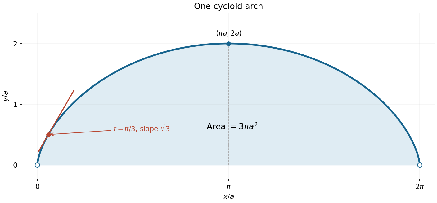
Codex 0 2026-10-18Because along the arch, its area above the baseline is the definite integral . Changing to the parameter givesAdding or removing the two endpoint points does not change the area. This is the area formula in area and length of a cycloid arch.
Past exam of the mathematics course of the year 1 of the natural sciences course of the University of Cambridge 2015 Paper 1 14 c Solution by Codex 0 2026-10-18
Codex 0 2026-10-18 Past exam of the mathematics course of the year 1 of the natural sciences course of the University of Cambridge 2015 Paper 1 14 b Solution by Codex 0 2026-10-18
Codex 0 2026-10-18The cycloid has limiting endpoints and , with its highest point at . The transformation sends to and preserves , so the arch is symmetric about . Its slope decreases from through zero to , giving vertical limiting tangent lines at the cusps and a horizontal tangent line at the top. More explicitly,so the arch is a concave function throughout its interior. The endpoint cusps are limiting points, excluded by the open parameter interval.
Past exam of the mathematics course of the year 1 of the natural sciences course of the University of Cambridge 2015 Paper 1 14 a Solution by Codex 0 2026-10-18
Codex 0 2026-10-18 Past exam of the mathematics course of the year 1 of the natural sciences course of the University of Cambridge 2015 Paper 1 13 c Solution by Codex 0 2026-10-18
Codex 0 2026-10-18The heat equation is linear and homogeneous in : the operator satisfies . Thus the superposition principle applies to its solutions. Spatial translations are also allowed because the coefficients are constant.
Choose in part (b) and multiply by to make the initial amplitude one. Taking the two shifts and then givesAt this reproduces both initial peaks. Each term is an instance of Gaussian initial data for the heat equation, so their sum satisfies the equation. Its extension to negative times is a real smooth solution precisely on the connected intervalAt the lower endpoint the peaks narrow without bound and their heights diverge; there is no finite classical continuation there. For positive times each peak spreads and decreases in height while preserving its integral.
Past exam of the mathematics course of the year 1 of the natural sciences course of the University of Cambridge 2015 Paper 1 13 b Solution by Codex 0 2026-10-18
Codex 0 2026-10-18For a Gaussian function, the required derivatives areSubstitute these into the reduced ordinary differential equation and compare the constant and quadratic coefficients:The constant terms give , and this value also satisfies the quadratic terms. HenceA constant multiple is also a solution by linearity.
Past exam of the mathematics course of the year 1 of the natural sciences course of the University of Cambridge 2015 Paper 1 13 a Solution by Codex 0 2026-10-18
Codex 0 2026-10-18Set . The similarity solution uses , whose partial derivatives at fixed or areApply the multivariable chain rule to :Substituting in the heat equation and cancelling the positive common factor gives
Past exam of the mathematics course of the year 1 of the natural sciences course of the University of Cambridge 2015 Paper 1 12 b Solution by Codex 0 2026-10-18
Codex 0 2026-10-18The partial derivatives are and , so all stationary points are for integers . Their Hessian matrix is . At even multiples of it is a positive-definite matrix, whereas at odd multiples it has one positive and one negative eigenvalue. ConsequentlyThere are no local maxima. Since both and are nonnegative, these are also global minima. In the requested open plotting window, the stationary points are and ; the local minima at lie on excluded edges.
For a level set , solving for the vertical coordinate givesFor these level sets are closed ovals around each local minimum. At the level sets shrink to the local minima. The level set through the saddle points iswhere the two signed branches together describe the same set as . They cross at and reach . The crossing slopes at a saddle point are , as also follows from the local quadratic form . For , the upper and lower level sets remain separate and extend across the plotting window without meeting the horizontal axis.
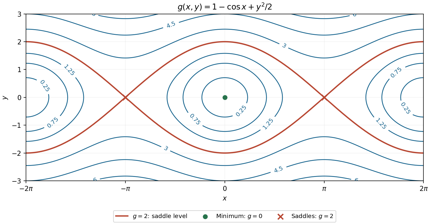
Contours of the cosine-plus-quadratic function, with its saddle level and stationary points labelled
. Details. Pinned article: Introduction to the OurBigBook Project
Welcome to the OurBigBook Project! Our goal is to create the perfect publishing platform for STEM subjects, and get university-level students to write the best free STEM tutorials ever.
Everyone is welcome to create an account and play with the site: ourbigbook.com/go/register. We belive that students themselves can write amazing tutorials, but teachers are welcome too. You can write about anything you want, it doesn't have to be STEM or even educational. Silly test content is very welcome and you won't be penalized in any way. Just keep it legal!
Intro to OurBigBook
. Source. We have two killer features:
- topics: topics group articles by different users with the same title, e.g. here is the topic for the "Fundamental Theorem of Calculus" ourbigbook.com/go/topic/fundamental-theorem-of-calculusArticles of different users are sorted by upvote within each article page. This feature is a bit like:
- a Wikipedia where each user can have their own version of each article
- a Q&A website like Stack Overflow, where multiple people can give their views on a given topic, and the best ones are sorted by upvote. Except you don't need to wait for someone to ask first, and any topic goes, no matter how narrow or broad
This feature makes it possible for readers to find better explanations of any topic created by other writers. And it allows writers to create an explanation in a place that readers might actually find it.
Figure 1. Screenshot of the "Derivative" topic page. View it live at: ourbigbook.com/go/topic/derivativeVideo 2. OurBigBook Web topics demo. Source. - local editing: you can store all your personal knowledge base content locally in a plaintext markup format that can be edited locally and published either:This way you can be sure that even if OurBigBook.com were to go down one day (which we have no plans to do as it is quite cheap to host!), your content will still be perfectly readable as a static site.
- to OurBigBook.com to get awesome multi-user features like topics and likes
- as HTML files to a static website, which you can host yourself for free on many external providers like GitHub Pages, and remain in full control

Figure 2. You can publish local OurBigBook lightweight markup files to either OurBigBook.com or as a static website.
Figure 3. Visual Studio Code extension installation.
Figure 5. . You can also edit articles on the Web editor without installing anything locally. Video 3. Edit locally and publish demo. Source. This shows editing OurBigBook Markup and publishing it using the Visual Studio Code extension. 
- Infinitely deep tables of contents:




All our software is open source and hosted at: github.com/ourbigbook/ourbigbook
Further documentation can be found at: docs.ourbigbook.com
Feel free to reach our to us for any help or suggestions: docs.ourbigbook.com/#contact